神经网络架构搜索-Neural Architecture Search

Search Space
Search Algorithms
Evaluation Strategy
One-Shot Approach: Search + Evaluation
What’s the Future?
Appendix: Summary of NAS Papers
Reference

Neural Architecture Search (NAS) automates network architecture engineering. It aims to learn a network topology that can achieve best performance on a certain task. By dissecting the methods for NAS into three components: search space, search algorithm and child model evolution strategy, this post reviews many interesting ideas for better, faster and more cost-efficient automatic neural architecture search.

原文：Neural Architecture Search
【2021-2-27】Lilian Weng：看过不少论文，里面提出的微小改变完全可以用一句话说清楚。该有种更好的方式来分享渐进式的改进和实验结果。有些论文很有趣，也很有价值，但写成十页似乎也太长了。

Although most popular and successful model architectures are designed by human experts, it doesn’t mean we have explored the entire network architecture space and settled down with the best option. We would have a better chance to find the optimal solution if we adopt a systematic and automatic way of learning high-performance model architectures.

Automatically learning and evolving network topologies is not a new idea (Stanley & Miikkulainen, 2002). In recent years, the pioneering work by Zoph & Le 2017 and Baker et al. 2017 has attracted a lot of attention into the field of Neural Architecture Search (NAS), leading to many interesting ideas for better, faster and more cost-efficient NAS methods.

As I started looking into NAS, I found this nice survey very helpful by Elsken, et al 2019. They characterize NAS as a system with three major components, which is clean & concise, and also commonly adopted in other NAS papers.

Search space: The NAS search space defines a set of operations (e.g. convolution, fully-connected, pooling) and how operations can be connected to form valid network architectures. The design of search space usually involves human expertise, as well as unavoidably human biases.
Search algorithm: A NAS search algorithm samples a population of network architecture candidates. It receives the child model performance metrics as rewards (e.g. high accuracy, low latency) and optimizes to generate high-performance architecture candidates.
Evaluation strategy: We need to measure, estimate, or predict the performance of a large number of proposed child models in order to obtain feedback for the search algorithm to learn. The process of candidate evaluation could be very expensive and many new methods have been proposed to save time or computation resources.

High-level categorization of NAS

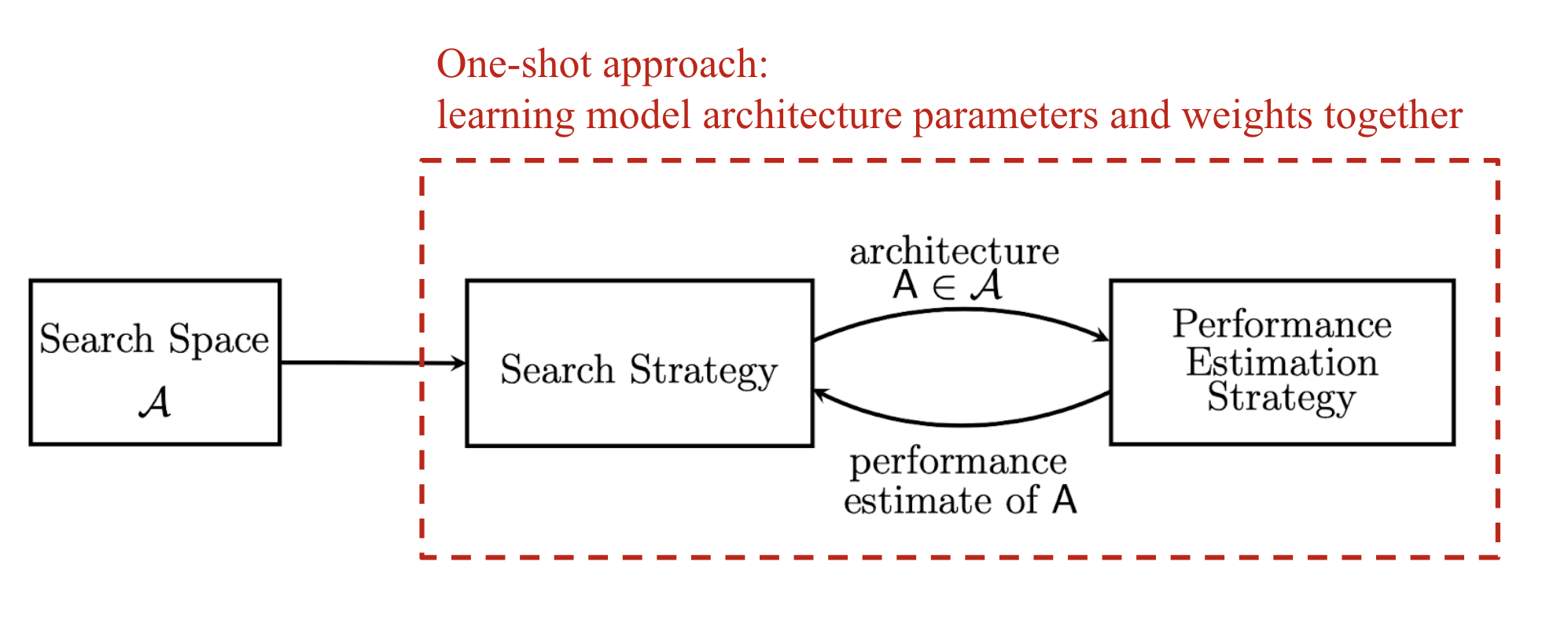
Fig. 1. Three main components of Neural Architecture Search (NAS) models. (Image source: Elsken, et al. 2019 with customized annotation in red)

Search Space

The NAS search space defines a set of basic network operations and how operations can be connected to construct valid network architectures.

Sequential Layer-wise Operations

The most naive way to design the search space for neural network architectures is to depict network topologies, either CNN or RNN, with a list of sequential layer-wise operations, as seen in the early work of Zoph & Le 2017 & Baker et al. 2017. The serialization of network representation requires a decent amount of expert knowledge, since each operation is associated with different layer-specific parameters and such associations need to be hardcoded. For example, after predicting a conv op, the model should output kernel size, stride size, etc; or after predicting an FC op, we need to see the number of units as the next prediction.

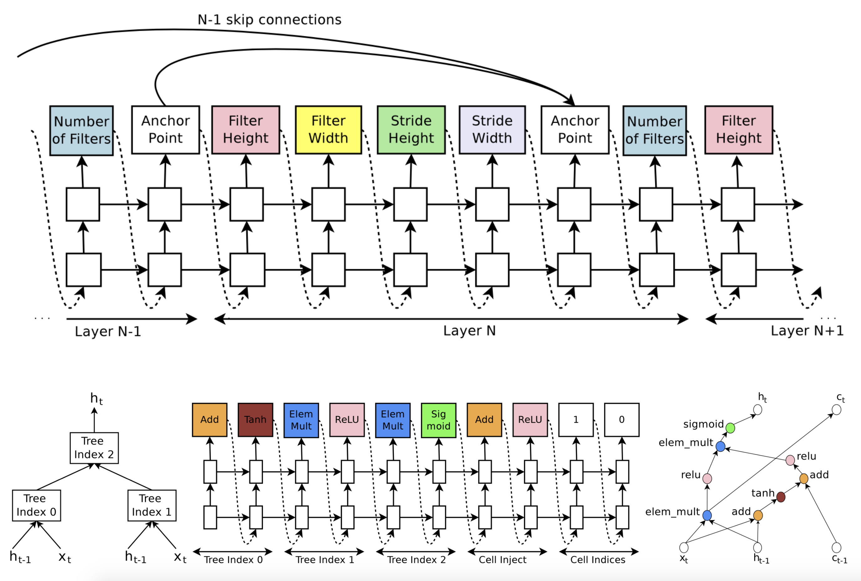
Fig. 2. (Top) A sequential representation of CNN. (Bottom) A sequential representation of the tree structure of a recurrent cell. (Image source: Zoph & Le 2017)

To make sure the generated architecture is valid, additional rules might be needed (Zoph & Le 2017):

If a layer is not connected to any input layer then it is used as the input layer;
At the final layer, take all layer outputs that have not been connected and concatenate them;
If one layer has many input layers, then all input layers are concatenated in the depth dimension;
If input layers to be concatenated have different sizes, we pad the small layers with zeros so that the concatenated layers have the same sizes.

The skip connection can be predicted as well, using an attention-style mechanism. At layer $i$ , an anchor point is added with $i−1$ content-based sigmoids to indicate which of the previous layers to be connected. Each sigmoid takes as input the hidden states of the current node $h_i$ and $i-1$ previous nodes $h_j, j=1, \dots, i-1$ .

\[P(\text{Layer j is an input to layer i}) = \text{sigmoid}(v^\top \tanh(\mathbf{W}_\text{prev} h_j + \mathbf{W}_\text{curr} h_i))\]

The sequential search space has a lot of representation power, but it is very large and consumes a ton of computation resources to exhaustively cover the search space. In the experiments by Zoph & Le 2017, they were running 800 GPUs in parallel for 28 days and Baker et al. 2017 restricted the search space to contain at most 2 FC layers.

Cell-based Representation

Inspired by the design of using repeated modules in successful vision model architectures (e.g. Inception, ResNet), the NASNet search space (Zoph et al. 2018) defines the architecture of a conv net as the same cell getting repeated multiple times and each cell contains several operations predicted by the NAS algorithm. A well-designed cell module enables transferability between datasets. It is also easy to scale down or up the model size by adjusting the number of cell repeats.

Precisely, the NASNet search space learns two types of cells for network construction:

Normal Cell: The input and output feature maps have the same dimension.
Reduction Cell: The output feature map has its width and height reduced by half.

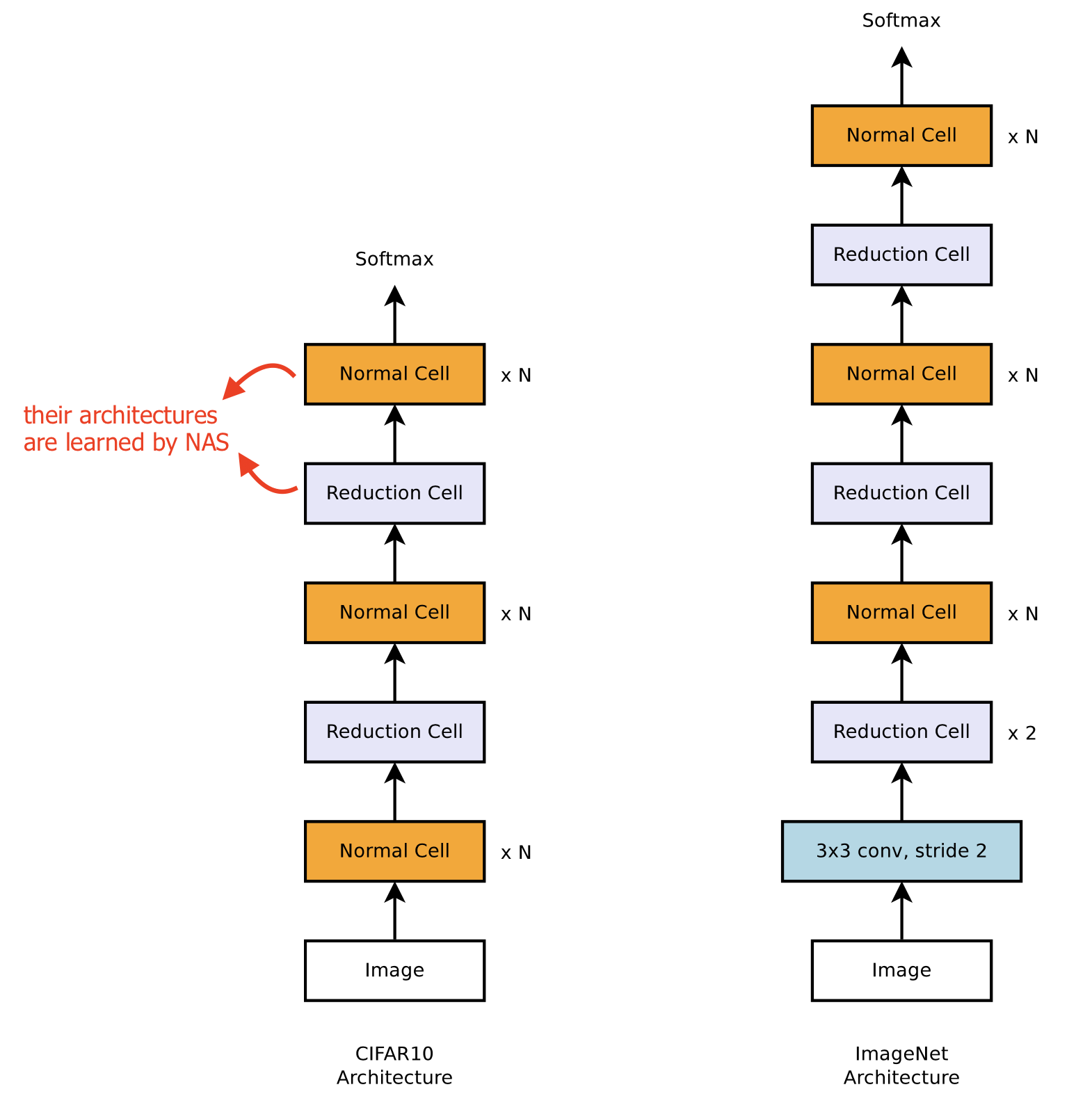
Fig. 3. The NASNet search space constrains the architecture as a repeated stack of cells. The cell architecture is optimized via NAS algorithms. (Image source: Zoph et al. 2018)

The predictions for each cell are grouped into $B$ blocks ($B=5$ in the NASNet paper), where each block has 5 prediction steps made by 5 distinct softmax classifiers corresponding to discrete choices of the elements of a block. Note that the NASNet search space does not have residual connections between cells and the model only learns skip connections on their own within blocks.

5 prediction steps in one block

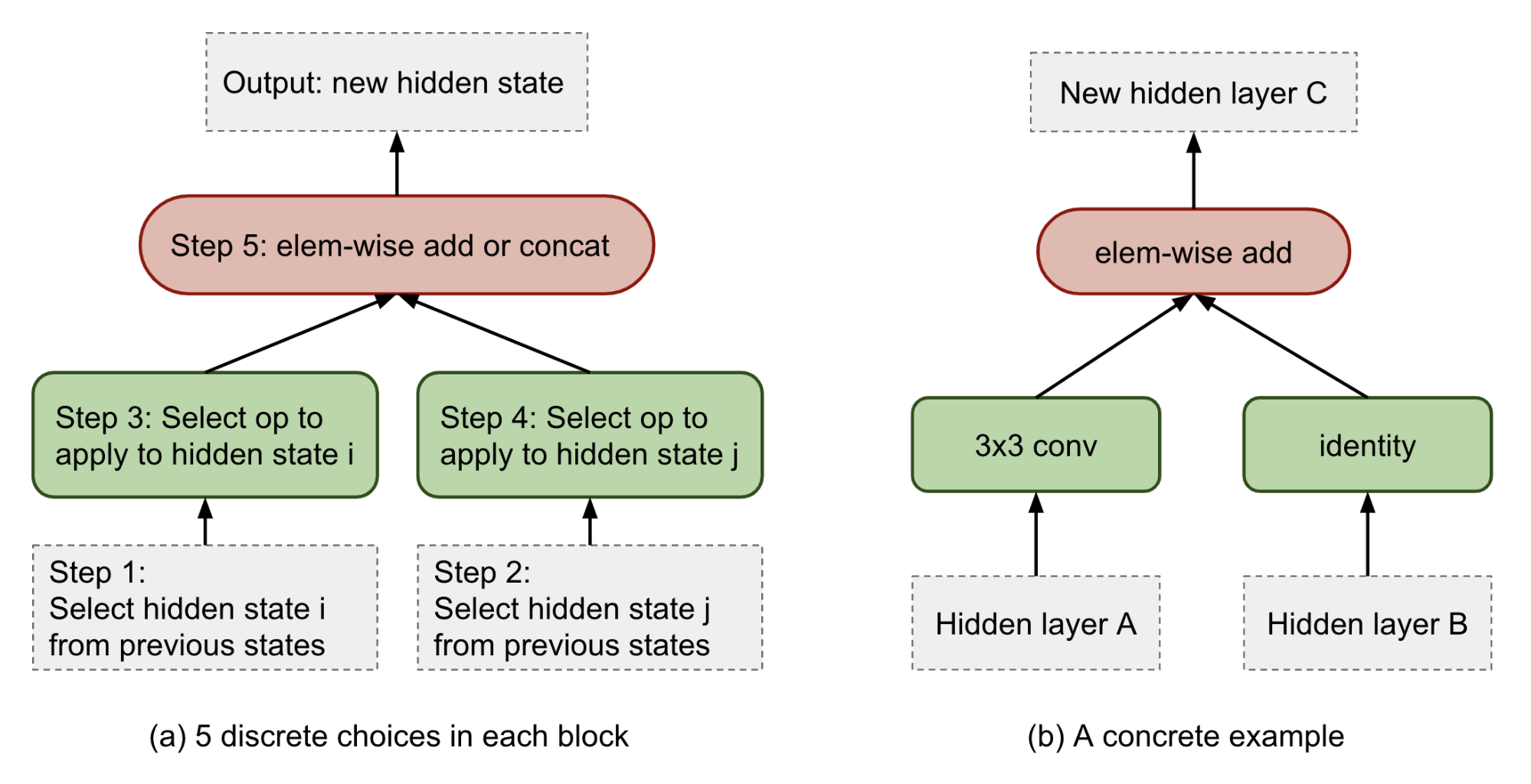
Fig. 4. (a) Each cell consists of $B$ blocks and each block is predicted by 5 discrete decisions. (b) An concrete example of what operations can be chosen in each decision step.

During the experiments, they discovered that a modified version of DropPath, named ScheduledDropPath, significantly improves the final performance of NASNet experiments. DropPath stochastically drops out paths (i.e. edges with operations attached in NASNet) with a fixed probability. ScheduledDropPath is DropPath with a linearly increasing probability of path dropping during training time.

Elsken, et al (2019) point out three major advantages of the NASNet search space:

The search space size is reduced drastically;
The motif-based architecture can be more easily transferred to different datasets.
It demonstrates a strong proof of a useful design pattern of repeatedly stacking modules in architecture engineering. For example, we can build strong models by stacking residual blocks in CNN or stacking multi-headed attention blocks in Transformer.

Hierarchical Structure

To take advantage of already discovered well-designed network motifs, the NAS search space can be constrained as a hierarchical structure, as in Hierarchical NAS (HNAS; (Liu et al 2017)). It starts with a small set of primitives, including individual operations like convolution operation, pooling, identity, etc. Then small sub-graphs (or “motifs”) that consist of primitive operations are recursively used to form higher-level computation graphs.

A computation motif at level $\ell=1, \dots, L$ can be represented by $(G^{(\ell)}, \mathcal{O}^{(\ell)})$, where:

$\mathcal{O}^{(\ell)}$ is a set of operations, $\mathcal{O}^{(\ell)} = \{ o^{(\ell)}_1, o^{(\ell)}_2, \dots \}$
$G^{(\ell)}$ is an adjacency matrix, where the entry $G_{ij}=k$ indicates that operation $o^{(\ell)}_k$ is placed between node $i$ and $j$. The node indices follow topological ordering in DAG, where the index $1$ is the source and the maximal index is the sink node.

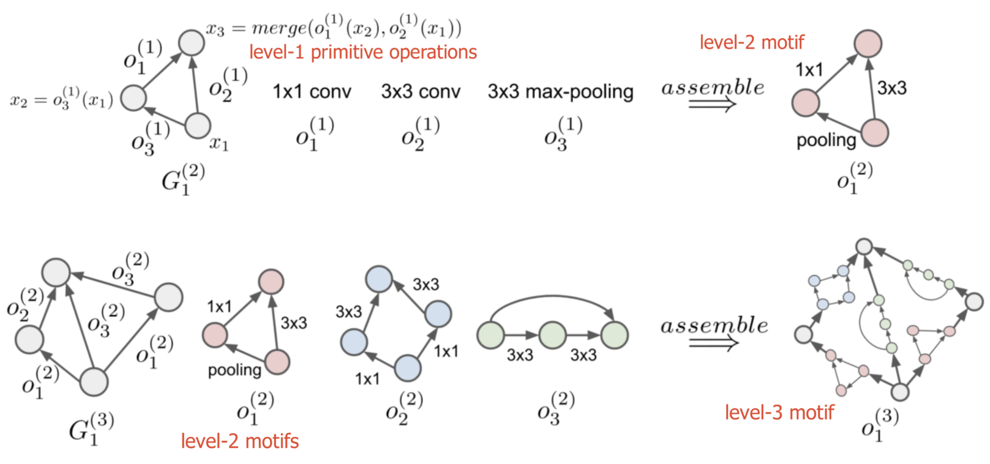
Fig. 5. (Top) Three level-1 primitive operations are composed into a level-2 motif. (Bottom) Three level-2 motifs are plugged into a base network structure and assembled into a level-3 motif. (Image source: Liu et al 2017)

To build a network according to the hierarchical structure, we start from the lowest level $\ell=1$ and recursively define the $m$-th motif operation at level $\ell$ as

\[o^{(\ell)}_m = \text{assemble}\Big( G_m^{(\ell)}, \mathcal{O}^{(\ell-1)} \Big)\]

A hierarchical representation becomes $\Big( \big\{ \{ G_m^{(\ell)} \}_{m=1}^{M_\ell} \big\}_{\ell=2}^L, \mathcal{O}^{(1)} \Big), \forall \ell=2, \dots, L$, where $\mathcal{O}^{(1)}$ contains a set of primitive operations.

The $\text{assemble}()$ process is equivalent to sequentially compute the feature map of node $i$ by aggregating all the feature maps of its predecessor node $j$ following the topological ordering:

\[x_i = \text{merge} \big[ \{ o^{(\ell)}_{G^{(\ell)}_{ij}}(x_j) \}_{j < i} \big], i = 2, \dots, \vert G^{(\ell)} \vert\]

where $\text{merge}[]$ is implemented as depth-wise concatenation in the paper.

Same as NASNet, experiments in Liu et al (2017) focused on discovering good cell architecture within a predefined “macro” structure with repeated modules. They showed that the power of simple search methods (e.g. random search or evolutionary algorithms) can be substantially enhanced using well-designed search spaces.

Cai et al (2018b) propose a tree-structure search space using path-level network transformation. Each node in a tree structure defines an allocation scheme for splitting inputs for child nodes and a merge scheme for combining results from child nodes. The path-level network transformation allows replacing a single layer with a multi-branch motif if its corresponding merge scheme is add or concat.

Path-level network transformation

Fig. 6. An illustration of transforming a single layer to a tree-structured motif via path-level transformation operations. (Image source: Cai et al. 2018b)

Memory-bank Representation

A memory-bank representation of feed-forward networks is proposed by Brock et al. (2017) in SMASH. Instead of a graph of operations, they view a neural network as a system with multiple memory blocks which can read and write. Each layer operation is designed to: (1) read from a subset of memory blocks; (2) computes results; finally (3) write the results into another subset of blocks. For example, in a sequential model, a single memory block would get read and overwritten consistently.

Memory-bank representation

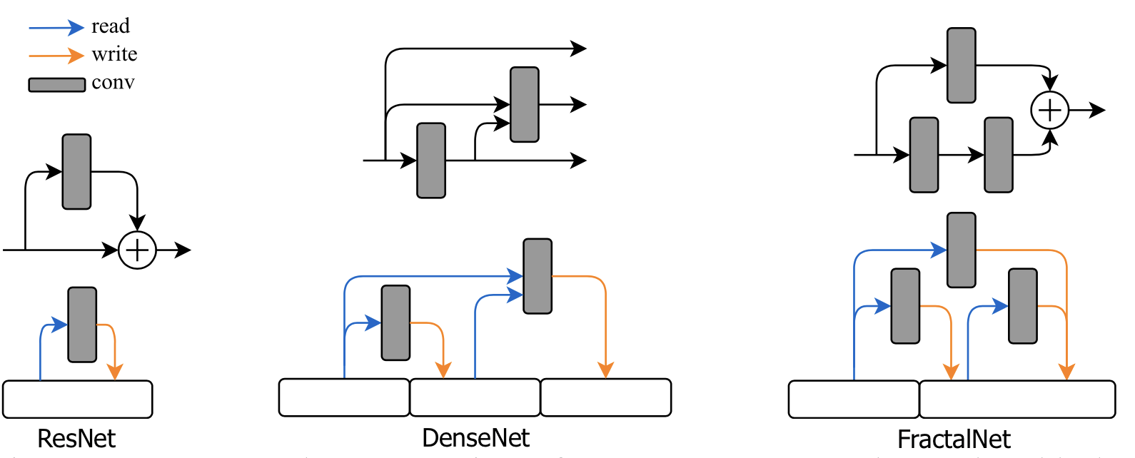
Fig. 7. Memory-bank representation of several popular network architecture blocks. (Image source: Brock et al. 2017)

Search Algorithms

NAS search algorithms sample a population of child networks. It receives the child models’ performance metrics as rewards and learns to generate high-performance architecture candidates. You may a lot in common with the field of hyperparameter search.

Random Search

Random search is the most naive baseline. It samples a valid architecture candidate from the search space at random and no learning model is involved. Random search has proved to be quite useful in hyperparameter search (Bergstra & Bengio 2012). With a well-designed search space, random search could be a very challenging baseline to beat.

Reinforcement Learning

The initial design of NAS (Zoph & Le 2017) involves a RL-based controller for proposing child model architectures for evaluation. The controller is implemented as a RNN, outputting a variable-length sequence of tokens used for configuring a network architecture.

NAS

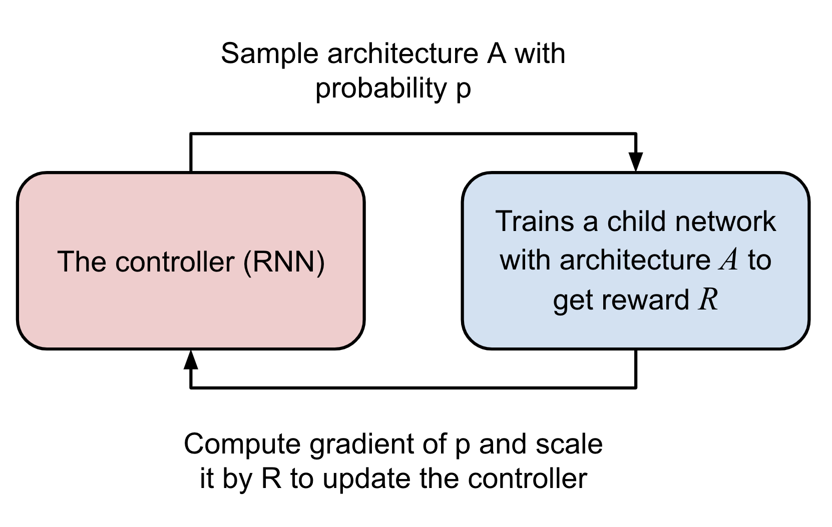
Fig. 8. A high level overview of NAS, containing a RNN controller and a pipeline for evaluating child models. (Image source: Zoph & Le 2017)

The controller is trained as a RL task using REINFORCE.

Action space: The action space is a list of tokens for defining a child network predicted by the controller (See more in the above section). The controller outputs action, $a_{1:T}$, where $T$ is the total number of tokens.
Reward: The accuracy of a child network that can be achieved at convergence is the reward for training the controller, $R$.
Loss: NAS optimizes the controller parameters $\theta$ with a REINFORCE loss. We want to maximize the expected reward (high accuracy) with the gradient as follows. The nice thing here with policy gradient is that it works even when the reward is non-differentiable.

\[\nabla_{\theta} J(\theta) = \sum_{t=1}^T \mathbb{E}[\nabla_{\theta} \log P(a_t \vert a_{1:(t-1)}; \theta) R ]\]

MetaQNN (Baker et al. 2017) trains an agent to sequentially choose CNN layers using Q-learning with an $\epsilon$-greedy exploration strategy and experience replay. The reward is the validation accuracy as well.

\[Q^{(t+1)}(s_t, a_t) = (1 - \alpha)Q^{(t)}(s_t, a_t) + \alpha (R_t + \gamma \max_{a \in \mathcal{A}} Q^{(t)}(s_{t+1}, a'))\]

where a state $s_t$ is a tuple of layer operation and related parameters. An action $$a$ determines the connectivity between operations. The Q-value is proportional to how confident we are in two connected operations leading to high accuracy.

MetaQNN

Fig. 9. Overview of MetaQNN - designing CNN models with Q-Learning. (Image source: Baker et al. 2017)

Evolutionary Algorithms

NEAT (short for NeuroEvolution of Augmenting Topologies) is an approach for evolving neural network topologies with genetic algorithm (GA), proposed by Stanley & Miikkulainen in 2002. NEAT evolves both connection weights and network topology together. Each gene encodes the full information for configuring a network, including node weights and edges. The population grows by applying mutation of both weights and connections, as well as crossover between two parent genes. For more in neuroevolution, please refer to the in-depth survey by Stanley et al. (2019).

Mutation operations in NEAT

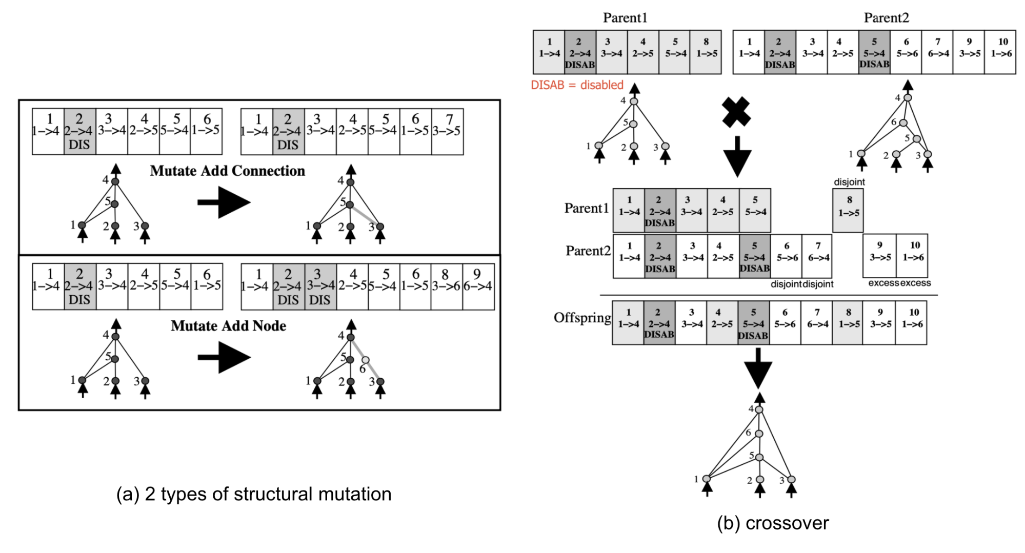
Fig. 10. Mutations in the NEAT algorithm. (Image source: Fig 3 & 4 in Stanley & Miikkulainen, 2002)

Real et al. (2018) adopt the evolutionary algorithms (EA) as a way to search for high-performance network architectures, named AmoebaNet. They apply the tournament selection method, which at each iteration picks a best candidate out of a random set of samples and places its mutated offspring back into the population. When the tournament size is $1$, it is equivalent to random selection.

AmoebaNet modified the tournament selection to favor younger genotypes and always discard the oldest models within each cycle. Such an approach, named aging evolution, allows AmoebaNet to cover and explore more search space, rather than to narrow down on good performance models too early.

Precisely, in every cycle of the tournament selection with aging regularization (See Figure 11):

Sample $S$ models from the population and the one with highest accuracy is chosen as parent.
A child model is produced by mutating parent.
Then the child model is trained, evaluated and added back into the population.
The oldest model is removed from the population.

Aging evolution algorithm

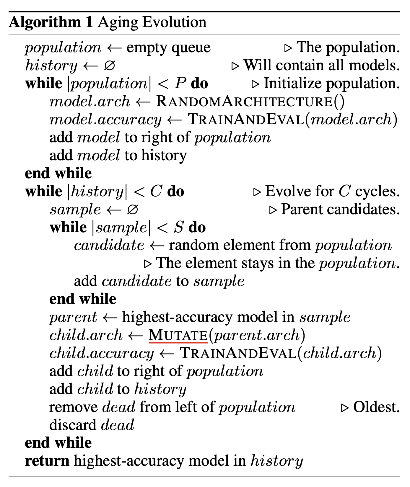
Fig. 11. The algorithm of aging evolution. (Image source: Real et al. 2018)

Two types of mutations are applied:

Hidden state mutation: randomly chooses a pairwise combination and rewires a random end such that there is no loop in the graph.
Operation mutation: randomly replaces an existing operation with a random one.

Mutations in AmoebaNet

Fig. 12. Two types of mutations in AmoebaNet. (Image source: Real et al. 2018)

In their experiments, EA and RL work equally well in terms of the final validation accuracy, but EA has better anytime performance and is able to find smaller models. Here using EA in NAS is still expensive in terms of computation, as each experiment took 7 days with 450 GPUs.

HNAS (Liu et al 2017) also employs the evolutionary algorithms (the original tournament selection) as their search strategy. In the hierarchical structure search space, each edge is an operation. Thus genotype mutation in their experiments is applied by replacing a random edge with a different operation. The replacement set includes an none op, so it can alter, remove and add an edge. The initial set of genotypes is created by applying a large number of random mutations on “trivial” motifs (all identity mappings).

Progressive Decision Process

Constructing a model architecture is a sequential process. Every additional operator or layer brings extra complexity. If we guide the search model to start the investigation from simple models and gradually evolve to more complex architectures, it is like to introduce “curriculum” into the search model’s learning process.

Progressive NAS (PNAS; Liu, et al 2018) frames the problem of NAS as a progressive procedure for searching models of increasing complexity. Instead of RL or EA, PNAS adopts a Sequential Model-based Bayesian Optimization (SMBO) as the search strategy. PNAS works similar to A* search, as it searches for models from simple to hard while simultaneously learning a surrogate function to guide the search.

A* search algorithm (“best-first search”) is a popular algorithm for path finding. The problem is framed as finding a path of smallest cost from a specific starting node to a given target node in a weighted graph. At each iteration, A* finds a path to extend by minimizing: $f(n)=g(n)+h(n)$, where $n$ is the next node, $g(n)$ is the cost from start to $n$, and $h(n)$ is the heuristic function that estimates the minimum cost of going from node $n$ to the goal.

PNAS uses the NASNet search space. Each block is specified as a 5-element tuple and PNAS only considers the element-wise addition as the step 5 combination operator, no concatenation. Differently, instead of setting the number of blocks $B$ at a fixed number, PNAS starts with $B=1$, a model with only one block in a cell, and gradually increases $B$.

The performance on a validation set is used as feedback to train a surrogate model for predicting the performance of novel architectures. With this predictor, we can thus decide which models should be prioritized to be evaluated next. Since the performance predictor should be able to handle various-sized inputs, accuracy, and sample-efficient, they ended up using an RNN model.

Progressive NAS

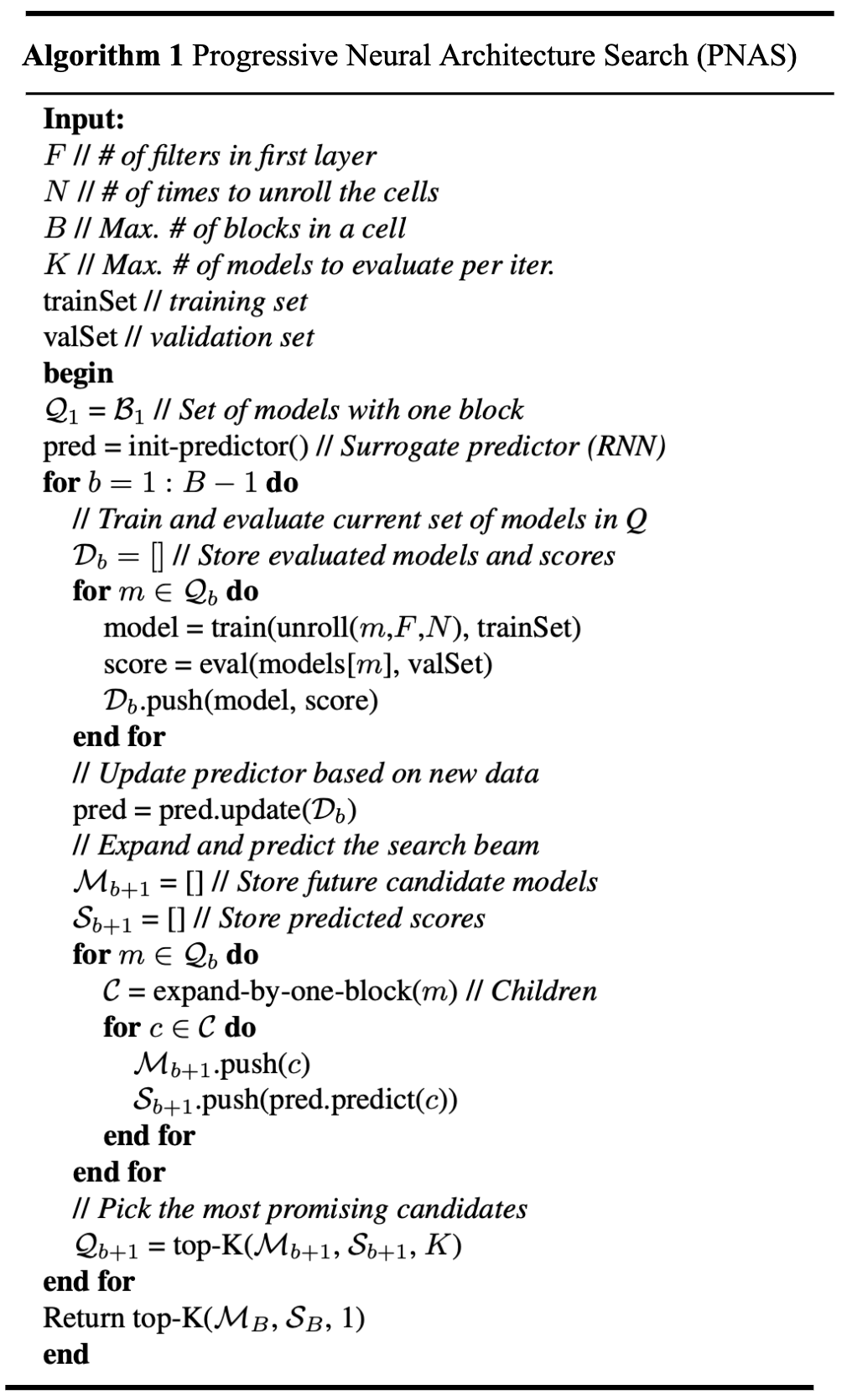
Fig. 13. The algorithm of Progressive NAS. (Image source: Liu, et al 2018)

Gradient descent

Using gradient descent to update the architecture search model requires an effort to make the process of choosing discrete operations differentiable. These approaches usually combine the learning of both architecture parameters and network weights together into one model. See more in the section on the “one-shot” approach.

Evaluation Strategy

We need to measure, estimate or predict the performance of every child model in order to obtain feedback for optimizing the search algorithm. The process of candidate evaluation could be very expensive and many new evaluation methods have been proposed to save time or computation. When evaluating a child model, we mostly care about its performance measured as accuracy on a validation set. Recent work has started looking into other factors of a model, such as model size and latency, as certain devices may have limitations on memory or demand fast response time.

Training from Scratch

The most naive approach is to train every child network independently from scratch until convergence and then measure its accuracy on a validation set (Zoph & Le 2017). It provides solid performance numbers, but one complete train-converge-evaluate loop only generates a single data sample for training the RL controller (let alone RL is known to be sample-inefficient in general). Thus it is very expensive in terms of computation consumption.

Proxy Task Performance

There are several approaches for using a proxy task performance as the performance estimator of a child network, which is generally cheaper and faster to calculate:

Train on a smaller dataset.
Train for fewer epochs.
Train and evaluate a down-scaled model in the search stage. For example, once a cell structure is learned, we can play with the number of cell repeats or scale up the number of filters (Zoph et al. 2018).
Predict the learning curve. Baker et al (2018) model the prediction of validation accuracies as a time-series regression problem. The features for the regression model ($\nu$-support vector machine regressions; $\nu$-SVR) include the early sequences of accuracy per epoch, architecture parameters, and hyperparameters.

Instead of training every child model independently from scratch. You may ask, ok, what if we fabricate dependency between them and find a way to reuse weights? Some researchers succeeded to make such approaches work.

Inspired by Net2net transformation, Cai et al (2017) proposed Efficient Architecture Search (EAS). EAS sets up an RL agent, known as a meta-controller, to predict function-preserving network transformation so as to grow the network depth or layer width. Because the network is growing incrementally, the weights of previously validated networks can be reused for further exploration. With inherited weights, newly constructed networks only need some light-weighted training.

A meta-controller learns to generate network transformation actions given the current network architecture, which is specified with a variable-length string. In order to handle architecture configuration of a variable length, the meta-controller is implemented as a bi-directional recurrent network. Multiple actor networks output different transformation decisions:

Net2WiderNet operation allows to replace a layer with a wider layer, meaning more units for fully-connected layers, or more filters for convolutional layers, while preserving the functionality.
Net2DeeperNet operation allows to insert a new layer that is initialized as adding an identity mapping between two layers so as to preserve the functionality.

EAS meta-controller

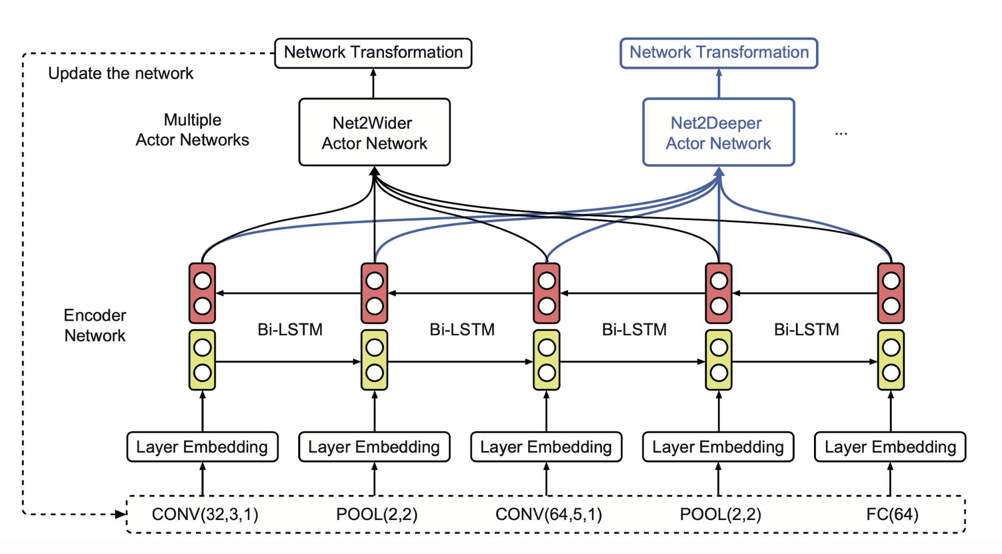
Fig. 14. Overview of the RL based meta-controller in Efficient Architecture Search (NAS). After encoding the architecture configuration, it outputs net2net transformation actions through two separate actor networks. (Image source: Cai et al 2017)

With similar motivation, Efficient NAS (ENAS; Pham et al. 2018) speeds up NAS (i.e. 1000x less) by aggressively sharing parameters among child models. The core motivation behind ENAS is the observation that all of the sampled architecture graphs can be viewed as sub-graphs of a larger supergraph. All the child networks are sharing weights of this supergraph.

ENAS example

Fig. 15. (Left) The graph represents the entire search space for a 4-node recurrent cell, but only connections in red are active. (Middle) An example of how the left active sub-graph can be translated into a child model architecture. (Right) The network parameters produced by an RNN controller for the architecture in the middle. (Image source: Pham et al. 2018)

ENAS alternates between training the shared model weights $\omega$ and training the controller $\theta$:

The parameters of the controller LSTM $\theta$ are trained with REINFORCE, where the reward $R(\mathbf{m}, \omega)$ is computed on the validation set.
The shared parameters of the child models $\omega$ are trained with standard supervised learning loss. Note that different operators associated with the same node in the supergraph would have their own distinct parameters.

Prediction-Based

A routine child model evaluation loop is to update model weights via standard gradient descent. SMASH (Brock et al. 2017) proposes a different and interesting idea: Can we predict the model weights directly based on the network architecture parameters?

They employ a HyperNet (Ha et al 2016) to directly generate the weights of a model conditioned on an encoding of its architecture configuration. Then the model with HyperNet-generated weights is validated directly. Note that we don’t need extra training for every child model but we do need to train the HyperNet.

SMASH algorithm

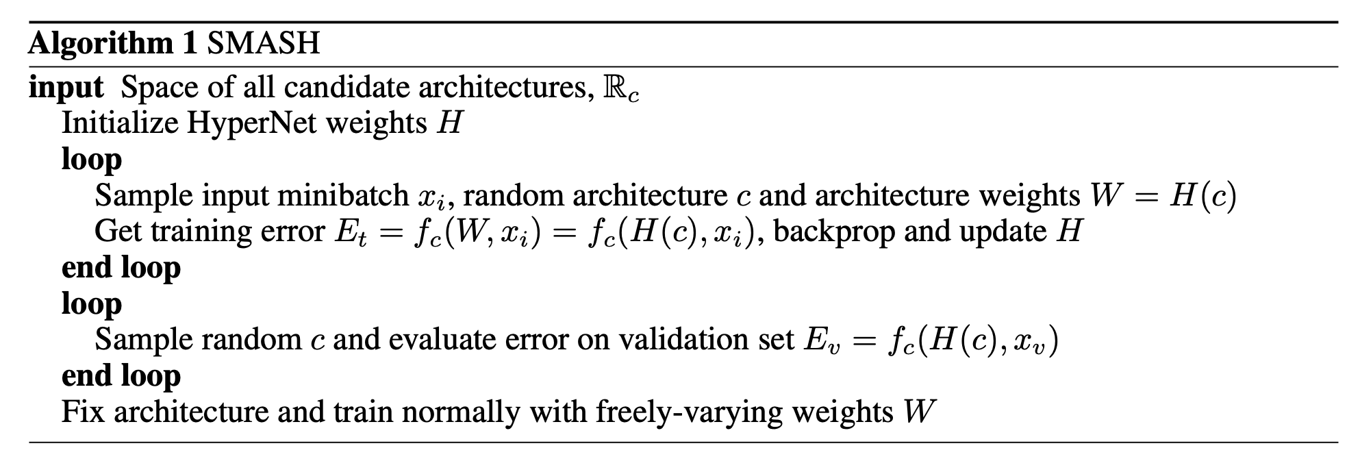
Fig. 16. The algorithm of SMASH. (Image source: Brock et al. 2017)

The correlation between model performance with SMASH-generated weights and true validation errors suggests that predicted weights can be used for model comparison, to some extent. We do need a HyperNet of large enough capacity, as the correlation would be corrupted if the HyperNet model is too small compared to the child model size.

SMASH error correlation

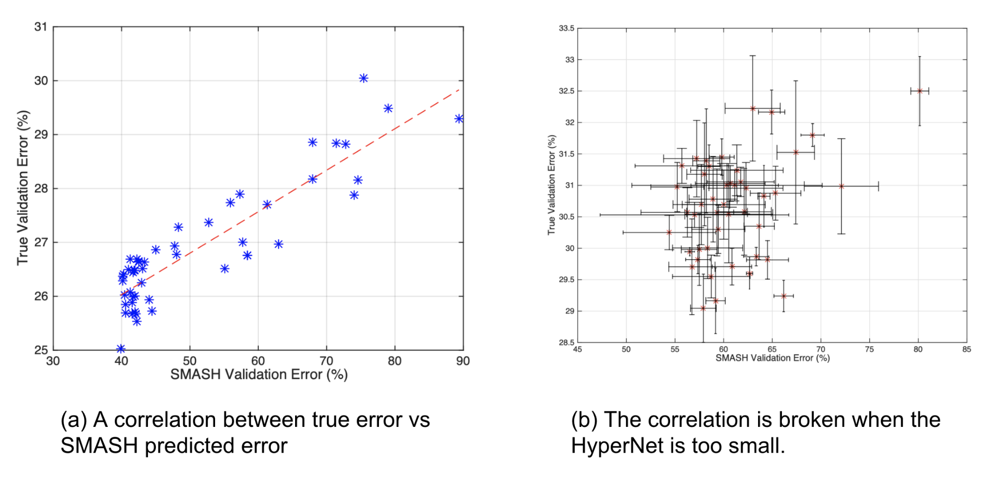
Fig. 17. The algorithm of SMASH. (Image source: Brock et al. 2017)

SMASH can be viewed as another way to implement the idea of parameter sharing. One problem of SMASH as pointed out by Pham et al. (2018) is: The usage of HyperNet restricts the weights of SMASH child models to a low-rank space, because weights are generated via tensor products. In comparison, ENAS has no such restrictions.

One-Shot Approach: Search + Evaluation

Running search & evaluation independently for a large population of child models is expensive. We have seen promising approaches like Brock et al. (2017) or Pham et al. (2018), where training a single model is enough for emulating any child model in the search space.

The one-shot architecture search extends the idea of weight sharing and further combines the learning of architecture generation together with weight parameters. The following approaches all treat child architectures as different sub-graphs of a supergraph with shared weights between common edges in the supergraph.

Bender et al (2018) construct a single large over-parameterized network, known as the One-Shot model, such that it contains every possible operation in the search space. With ScheduledDropPath (the dropout rate is increased over time, which is $r^{1/k}$ at the end of training, where $0 < r < 1$ is a hyperparam and $k$ is the number of incoming paths) and some carefully designed tricks (e.g. ghost batch normalization, L2 regularization only on the active architecture), the training of such a giant model can be stabilized enough and used for evaluating any child model sampled from the supergraph.

One-Shot model architecture

Fig. 18. The architecture of the One-Shot model in Bender et al 2018. Each cell has $N$ choice blocks and each choice block can select up to 2 operations. Solid edges are used in every architecture, where dash lines are optional. (Image source: Bender et al 2018)

Once the one-shot model is trained, it is used for evaluating the performance of many different architectures sampled at random by zeroing out or removing some operations. This sampling process can be replaced by RL or evolution.

They observed that the difference between the accuracy measured with the one-shot model and the accuracy of the same architecture after a small fine-tuning could be very large. Their hypothesis is that the one-shot model automatically learns to focus on the most useful operations in the network and comes to rely on these operations when they are available. Thus zeroing out useful operations lead to big reduction in model accuracy, while removing less important components only causes a small impact — Therefore, we see a larger variance in scores when using the one-shot model for evaluation.

One-shot accuracy

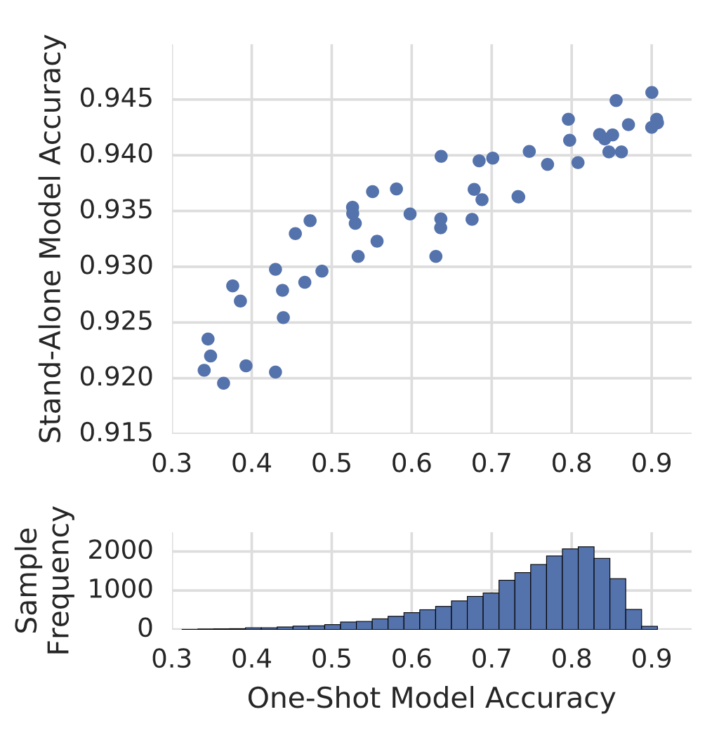
Fig. 19. A stratified sample of models with different one-shot model accuracy versus their true validation accuracy as stand-alone models. (Image source: Bender et al 2018)

Clearly designing such a search graph is not a trivial task, but it demonstrates a strong potential with the one-shot approach. It works well with only gradient descent and no additional algorithm like RL or EA is a must.

Some believe that one main cause for inefficiency in NAS is to treat the architecture search as a black-box optimization and thus we fall into methods like RL, evolution, SMBO, etc. If we shift to rely on standard gradient descent, we could potentially make the search process more effectively. As a result, Liu et al (2019) propose Differentiable Architecture Search (DARTS). DARTS introduces a continuous relaxation on each path in the search supergraph, making it possible to jointly train architecture parameters and weights via gradient descent.

Let’s use the directed acyclic graph (DAG) representation here. A cell is a DAG consisting of a topologically ordered sequence of $N$ nodes. Each node has a latent representation $x_i$ to be learned. Each edge $(i, j)$ is tied to some operation $o^{(i,j)} \in \mathcal{O}$ that transforms $x_j$ to compose $x_i$:

\[x_i = \sum_{j < i} o^{(i,j)}(x_j)\]

To make the search space continuous, DARTS relaxes the categorical choice of a particular operation as a softmax over all the operations and the task of architecture search is reduced to learn a set of mixing probabilities $\alpha = \{ \alpha^{(i,j)} \}$.

\[\bar{o}^{(i,j)}(x) = \sum_{o\in\mathcal{O}} \frac{\exp(\alpha_{ij}^o)}{\sum_{o'\in\mathcal{O}} \exp(\alpha^{o'}_{ij})} o(x)\]

where $\alpha_{ij}$ is a vector of dimension $\vert \mathcal{O} \vert$, containing weights between nodes $i$ and $j$ over different operations.

The bilevel optimization exists as we want to optimize both the network weights $w$ and the architecture representation $\alpha$:

\[\begin{aligned} \min_\alpha & \mathcal{L}_\text{validate} (w^*(\alpha), \alpha) \\ \text{s.t.} & w^*(\alpha) = \arg\min_w \mathcal{L}_\text{train} (w, \alpha) \end{aligned}\]

At step $k$, given the current architecture parameters $\alpha_{k−1}$, we first optimize weights $w_k$ by moving $w_{k−1}$ in the direction of minimizing the training loss $\mathcal{L}_\text{train}(w_{k−1}, \alpha_{k−1})$ with a learning rate $\xi$. Next, while keeping the newly updated weights $w_k$ fixed, we update the mixing probabilities so as to minimize the validation loss after a single step of gradient descent w.r.t. the weights:

\[J_\alpha = \mathcal{L}_\text{val}(w_k - \xi \nabla_w \mathcal{L}_\text{train}(w_k, \alpha_{k-1}), \alpha_{k-1})\]

The motivation here is that we want to find an architecture with a low validation loss when its weights are optimized by gradient descent and the one-step unrolled weights serve as the surrogate for $w^∗(\alpha)$.

Side note: Earlier we have seen similar formulation in MAML where the two-step optimization happens between task losses and the meta-learner update, as well as framing Domain Randomization as a bilevel optimization for better transfer in the real environment.

DARTS

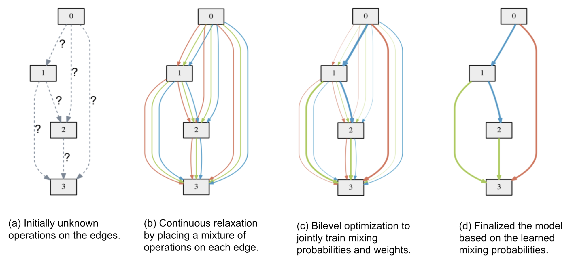
Fig. 20. An illustration of how DARTS applies continuous relaxation on edges in DAG supergraph and identifies the final model. (Image source: Liu et al 2019)

\[\begin{aligned} \text{Let }w'_k &= w_k - \xi \nabla_w \mathcal{L}_\text{train}(w_k, \alpha_{k-1}) & \\ J_\alpha &= \mathcal{L}_\text{val}(w_k - \xi \nabla_w \mathcal{L}_\text{train}(w_k, \alpha_{k-1}), \alpha_{k-1}) = \mathcal{L}_\text{val}(w'_k, \alpha_{k-1}) & \\ \nabla_\alpha J_\alpha &= \nabla_{\alpha_{k-1}} \mathcal{L}_\text{val}(w'_k, \alpha_{k-1}) \nabla_\alpha \alpha_{k-1} + \nabla_{w'_k} \mathcal{L}_\text{val}(w'_k, \alpha_{k-1})\nabla_\alpha w'_k & \\& \text{; multivariable chain rule}\\ &= \nabla_{\alpha_{k-1}} \mathcal{L}_\text{val}(w'_k, \alpha_{k-1}) + \nabla_{w'_k} \mathcal{L}_\text{val}(w'_k, \alpha_{k-1}) \big( - \xi \color{red}{\nabla^2_{\alpha, w} \mathcal{L}_\text{train}(w_k, \alpha_{k-1})} \big) & \\ &\approx \nabla_{\alpha_{k-1}} \mathcal{L}_\text{val}(w'_k, \alpha_{k-1}) - \xi \nabla_{w'_k} \mathcal{L}_\text{val}(w'_k, \alpha_{k-1}) \color{red}{\frac{\nabla_\alpha \mathcal{L}_\text{train}(w_k^+, \alpha_{k-1}) - \nabla_\alpha \mathcal{L}_\text{train}(w_k^-, \alpha_{k-1}) }{2\epsilon}} & \\ & \text{; apply numerical differentiation approximation} \end{aligned}\]

where the red part is using numerical differentiation approximation where $w_k^+ = w_k + \epsilon \nabla_{w'_k} \mathcal{L}_\text{val}(w'_k, \alpha_{k-1})$ and $w_k^- = w_k - \epsilon \nabla_{w'_k} \mathcal{L}_\text{val}(w'_k, \alpha_{k-1})$.

DARTS algorithm

Fig. 21. The algorithm overview of DARTS. (Image source: Liu et al 2019)

As another idea similar to DARTS, Stochastic NAS (Xie et al., 2019) applies a continuous relaxation by employing the concrete distribution (CONCRETE = CONtinuous relaxations of disCRETE random variables; Maddison et al 2017) and reparametrization tricks. The goal is same as DARTS, to make the discrete distribution differentiable and thus enable optimization by gradient descent.

DARTS is able to greatly reduce the cost of GPU hours. Their experiments for searching for CNN cells have $N=7$ and only took 1.5 days with a single GPU. However, it suffers from the high GPU memory consumption issue due to its continuous representation of network architecture. In order to fit the model into the memory of a single GPU, they picked a small $N$.

To constrain the GPU memory consumption, ProxylessNAS (Cai et al., 2019) views NAS as a path-level pruning process in DAG and binarizes the architecture parameters to force only one path to be active between two nodes at a time. The probabilities for an edge being either masked out or not are then learned by sampling a few binarized architectures and using BinaryConnect (Courbariaux et al., 2015) to update the corresponding probabilities. ProxylessNAS demonstrates a strong connection between NAS and model compression. By using path-level compression, it is able to save memory consumption by one order of magnitude.

Let’s continue with the graph representation. In a DAG adjacency matrix $G$ where $G_{ij}$ represents an edge between node $i$ and $j$ and its value can be chosen from the set of $\vert \mathcal{O} \vert$ candidate primitive operations, $\mathcal{O} = \{ o_1, \dots \}$. The One-Shot model, DARTS and ProxylessNAS all consider each edge as a mixture of operations, $m_\mathcal{O}$, but with different tweaks.

In One-Shot, $m_\mathcal{O}(x)$ is the sum of all the operations. In DARTS, it is a weighted sum where weights are softmax over a real-valued architecture weighting vector $\alpha$ of length $\vert \mathcal{O} \vert$. ProxylessNAS transforms the softmax probabilities of $\alpha$ into a binary gate and uses the binary gate to keep only one operation active at a time.

\[\begin{aligned} m^\text{one-shot}_\mathcal{O}(x) &= \sum_{i=1}^{\vert \mathcal{O} \vert} o_i(x) \\ m^\text{DARTS}_\mathcal{O}(x) &= \sum_{i=1}^{\vert \mathcal{O} \vert} p_i o_i(x) = \sum_{i=1}^{\vert \mathcal{O} \vert} \frac{\exp(\alpha_i)}{\sum_j \exp(\alpha_j)} o_i(x) \\ m^\text{binary}_\mathcal{O}(x) &= \sum_{i=1}^{\vert \mathcal{O} \vert} g_i o_i(x) = \begin{cases} o_1(x) & \text{with probability }p_1, \\ \dots &\\ o_{\vert \mathcal{O} \vert}(x) & \text{with probability }p_{\vert \mathcal{O} \vert} \end{cases} \\ \text{ where } g &= \text{binarize}(p_1, \dots, p_N) = \begin{cases} [1, 0, \dots, 0] & \text{with probability }p_1, \\ \dots & \\ [0, 0, \dots, 1] & \text{with probability }p_N. \\ \end{cases} \end{aligned}\]

Training steps of ProxylessNAS

Fig. 22. ProxylessNAS has two training steps running alternatively. (Image source: Cai et al., 2019)

ProxylessNAS runs two training steps alternatively:

When training weight parameters $w$, it freezes the architecture parameters $\alpha$ and stochastically samples binary gates $g$ according to the above $m^\text{binary}_\mathcal{O}(x)$. The weight parameters can be updated with standard gradient descent.
When training architecture parameters $\alpha$, it freezes $w$, resets the binary gates and then updates $\alpha$ on the validation set. Following the idea of BinaryConnect, the gradient w.r.t. architecture parameters can be approximately estimated using $\partial \mathcal{L} / \partial g_i$ in replacement for $\partial \mathcal{L} / \partial p_i$:

\[\begin{aligned} \frac{\partial \mathcal{L}}{\partial \alpha_i} &= \sum_{j=1}^{\vert \mathcal{O} \vert} \frac{\partial \mathcal{L}}{\partial p_j} \frac{\partial p_j}{\partial \alpha_i} \approx \sum_{j=1}^{\vert \mathcal{O} \vert} \frac{\partial \mathcal{L}}{\partial g_j} \frac{\partial p_j}{\partial \alpha_i} = \sum_{j=1}^{\vert \mathcal{O} \vert} \frac{\partial \mathcal{L}}{\partial g_j} \frac{\partial \frac{e^{\alpha_j}}{\sum_k e^{\alpha_k}}}{\partial \alpha_i} \\ &= \sum_{j=1}^{\vert \mathcal{O} \vert} \frac{\partial \mathcal{L}}{\partial g_j} \frac{\sum_k e^{\alpha_k} (\mathbf{1}_{i=j} e^{\alpha_j}) - e^{\alpha_j} e^{\alpha_i} }{(\sum_k e^{\alpha_k})^2} = \sum_{j=1}^{\vert \mathcal{O} \vert} \frac{\partial \mathcal{L}}{\partial g_j} p_j (\mathbf{1}_{i=j} -p_i) \end{aligned}\]

Instead of BinaryConnect, REINFORCE can also be used for parameter updates with the goal for maximizing the reward, while no RNN meta-controller is involved.

Computing $\partial \mathcal{L} / \partial g_i$ needs to calculate and store $o_i(x)$, which requires $\vert \mathcal{O} \vert$ times GPU memory. To resolve this issue, they factorize the task of choosing one path out of $N$ into multiple binary selection tasks (Intuition: “if a path is the best choice, it should be better than any other path”). At every update step, only two paths are sampled while others are masked. These two selected paths are updated according to the above equation and then scaled properly so that other path weights are unchanged. After this process, one of the sampled paths is enhanced (path weight increases) and the other is attenuated (path weight decreases), while all other paths stay unaltered.

Besides accuracy, ProxylessNAS also considers latency as an important metric to optimize, as different devices might have very different requirements on inference time latency (e.g. GPU, CPU, mobile). To make latency differentiable, they model latency as a continuous function of the network dimensions. The expected latency of a mixed operation can be written as $\mathbb{E}[\text{latency}] = \sum_j p_j F(o_j)$, where $F(.)$ is a latency prediction model:

proxylessNAS latency

Fig. 23. Add a differentiable latency loss into the training of ProxylessNAS. (Image source: Cai et al., 2019)

What’s the Future?

So far we have seen many interesting new ideas on automating the network architecture engineering through neural architecture search and many have achieved very impressive performance. However, it is a bit hard to do inference on why some architecture work well and how we can develop modules generalizable across tasks rather than being very dataset-specific.

As also noted in Elsken, et al (2019):

“…, so far it provides little insights into why specific architectures work well and how similar the architectures derived in independent runs would be. Identifying common motifs, providing an understanding why those motifs are important for high performance, and investigating if these motifs generalize over different problems would be desirable.”

In the meantime, purely focusing on improvement over validation accuracy might not be enough (Cai et al., 2019). Devices like mobile phones for daily usage in general have limited memory and computation power. While AI applications are on the way to affect our daily life, it is unavoidable to be more device-specific.

Another interesting investigation is to consider unlabelled dataset and self-supervised learning for NAS. The size of labelled dataset is always limited and it is not easy to tell whether such a dataset has biases or big deviation from the real world data distribution.

Liu et al (2020) delve into the question “Can we find high-quality neural architecture without human-annotated labels?” and proposed a new setup called Unsupervised Neural Architecture Search (UnNAS). The quality of the architecture needs to be estimated in an unsupervised fashion during the search phase. The paper experimented with three unsupervised pretext tasks: image rotation prediction, colorization, and solving the jigsaw puzzle.

They observed in a set of UnNAS experiments that:

High rank correlation between supervised accuracy and pretext accuracy on the same dataset. Typically the rank correlation is higher than 0.8, regardless of the dataset, the search space, and the pretext task.
High rank correlation between supervised accuracy and pretext accuracy across datasets.
Better pretext accuracy translates to better supervised accuracy.
Performance of UnNAS architecture is comparable to supervised counterparts, though not better yet.

One hypothesis is that the architecture quality is correlated with image statistics. Because CIFAR-10 and ImageNet are all on the natural images, they are comparable and the results are transferable. UnNAS could potentially enable a much larger amount of unlabelled data into the search phase which captures image statistics better.

Hyperparameter search is a long-standing topic in the ML community. And NAS automates architecture engineering. Gradually we are trying to automate processes in ML which usually demand a lot of human efforts. Taking even one more step further, is it possible to automatically discover ML algorithms? AutoML-Zero (Real et al 2020) investigates this idea. Using aging evolutionary algorithms, AutoML-Zero automatically searches for whole ML algorithms using little restriction on the form with only simple mathematical operations as building blocks.

It learns three component functions. Each function only adopts very basic operations.

Setup: initialize memory variables (weights).
Learn: modify memory variables
Predict: make a prediction from an input $x$.

AutoML-zero evaluation

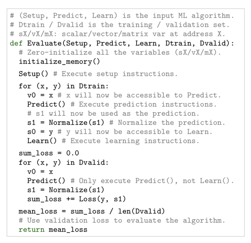
Fig. 24. Algorithm evaluation on one task (Image source: Real et al 2020)

Three types of operations are considered when mutating a parent genotype:

Insert a random instruction or remove an instruction at a random location in a component function;
Randomize all the instructions in a component function;
Modify one of the arguments of an instruction by replacing it with a random choice (e.g. “swap the output address” or “change the value of a constant”)

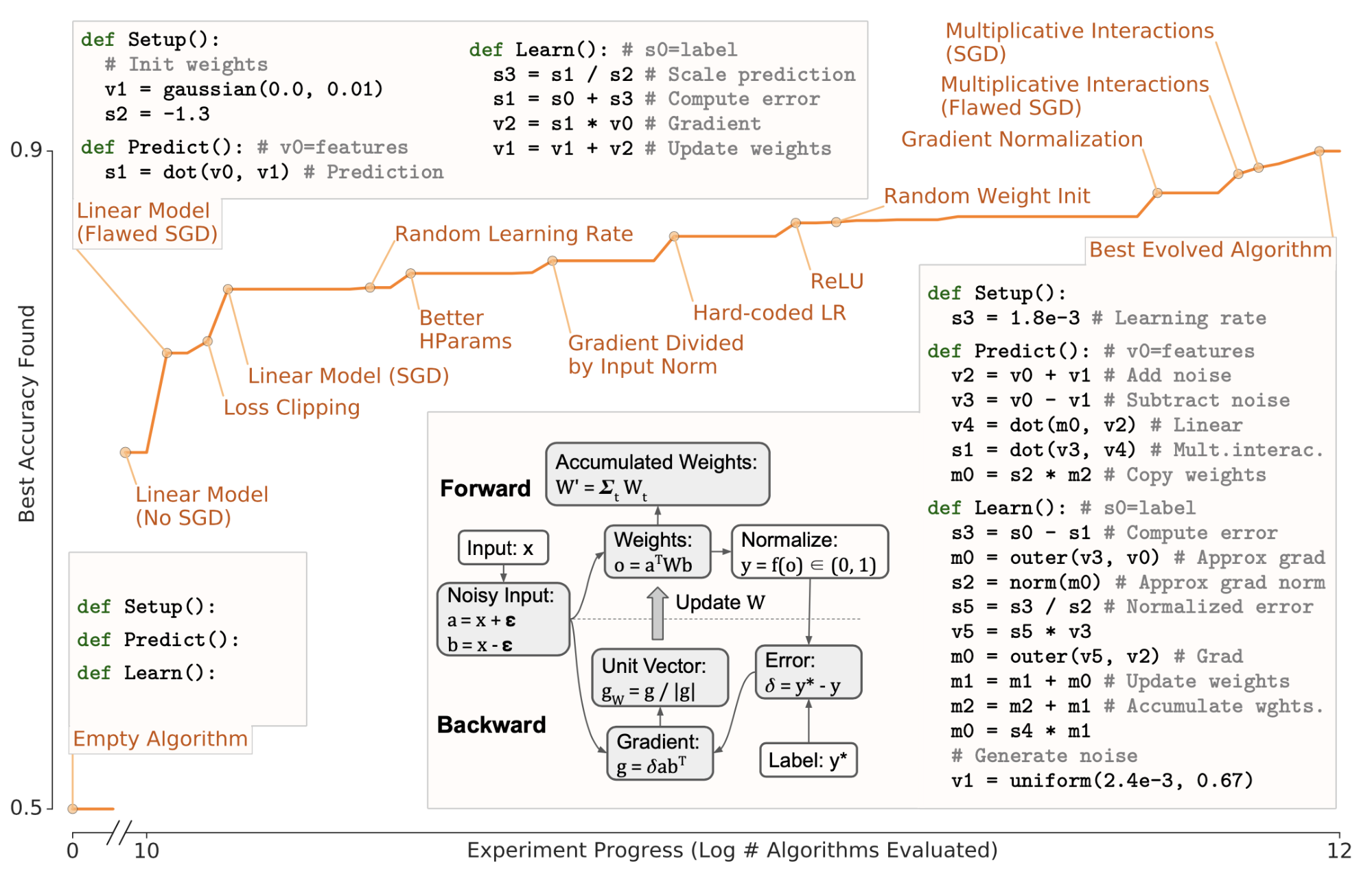
Progress of AutoML-zero experiment

Fig. 25. An illustration of evolutionary progress on projected binary CIFAR-10 with example code. (Image source: Real et al 2020)

Cited as:

@article{weng2020nas,
  title   = "Neural Architecture Search",
  author  = "Weng, Lilian",
  journal = "lilianweng.github.io/lil-log",
  year    = "2020",
  url     = "https://lilianweng.github.io/lil-log/2020/08/06/neural-architecture-search.html"
}

Appendix: Summary of NAS Papers

Model name	Search space	Search algorithms	Child model evaluation
NEAT (2002)	-	Evolution (Genetic algorithm)	-
NAS (2017)	Sequential layer-wise ops	RL (REINFORCE)	Train from scratch until convergence
MetaQNN (2017)	Sequential layer-wise ops	RL (Q-learning with $\epsilon$-greedy)	Train for 20 epochs
HNAS (2017)	Hierarchical structure	Evolution (Tournament selection)	Train for a fixed number of iterations
NASNet (2018)	Cell-based	RL (PPO)	Train for 20 epochs
AmoebaNet (2018)	NASNet search space	Evolution (Tournament selection with aging regularization)	Train for 25 epochs
EAS (2018a)	Network transformation	RL (REINFORCE)	2-stage training
PNAS (2018)	Reduced version of NASNet search space	SMBO; Progressive search for architectures of increasing complexity	Train for 20 epochs
ENAS (2018)	Both sequential and cell-based search space	RL (REINFORCE)	Train one model with shared weights
SMASH (2017)	Memory-bank representation	Random search	HyperNet predicts weights of evaluated architectures.
One-Shot (2018)	An over-parameterized one-shot model	Random search (zero out some paths at random)	Train the one-shot model
DARTS (2019)	NASNet search space	Gradient descent (Softmax weights over operations)
ProxylessNAS (2019)	Tree structure architecture	Gradient descent (BinaryConnect) or REINFORCE
SNAS (2019)	NASNet search space	Gradient descent (concrete distribution)