- 总结
- Few shot learning 小样本学习
- Meta-Learning 元学习
- Papers and Code
- Tutorials and Slides
- Reseachers and Labs
总结
- 【2021-2-5】阿里小蜜-北京 小样本学习(Few-shot Learning)综述
- 将 Few-shot Learning 和 Capsule Network 融合,提出了 Induction Network,在文本分类上做到了新的 state-of-the-art。
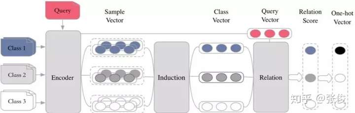
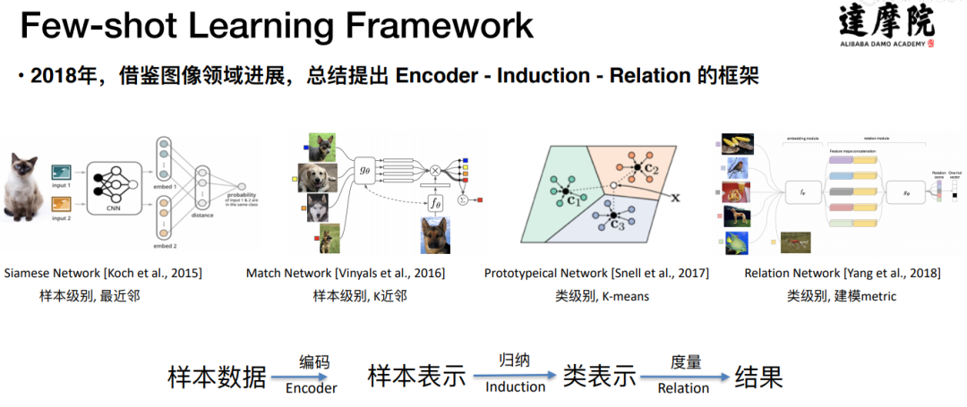
- 基于目前 Metric Based 方法,提出了 Encoder-Induction-Relation 的三级框架,如图 10 所示,Encoder 模块用于获取每个样本的语义表示,可以使用典型的 CNN、LSTM、Transformer 等结构,Induction 模块用于从支撑集的样本语义中归纳出类别特征,Relation 模块用于度量 query 和类别之间的语义关系,进而完成分类。
- 最新《小样本学习(Few-shot learning)》2020综述,34页pdf166篇参考文献
- 小样本学习综述《Generalizing from a Few Examples: A Survey on Few-Shot Learning》,包含166篇参考文献,来自第四范式和香港科技大学习的研究学者。
- Few-shot learning(少样本学习)入门
- 【2021-3-4】用于表格推理的小样本学习
- 发表于 Findings of EMNLP 2020 的“ 通过中间预训练以了解表格(Understanding tables with intermediate pre-training)”中,我们介绍了为表格解析定制的首批预训练任务,可使模型从更少的数据中更好、更快地学习
- 在较早的 TAPAS 模型基础上进行了改进,该模型是 BERT 双向 Transformer 模型的扩展,采用特殊嵌入向量在表格中寻找答案。新的预训练目标应用于 TAPAS 后即在涉及表格的多个数据集上达成突破性进展。
- 在 TabFact 上,它将模型和人类之间的表现差距缩小了约 50%。我们还系统地对选择相关输入的方法进行了基准测试以获得更高效率,实现了速度和内存的 4 倍提升,同时保留了 92% 的结果。适用于不同任务和规模的所有模型均已发布在 GitHub repo 中,您可以在 Colab Notebook 中试用它们。
- 引入了两个新的预训练二元分类任务,称其为反事实和合成任务,可以用作预训练的第二阶段(通常称为中间预训练),提高模型在表格数据上的性能
- 书籍: Hands-On Meta Learning With Python, 包含配套代码,Learning to Learn using One-Shot Learning, MAML, Reptile, Meta-SGD and more. You will delve into various one-shot learning algorithms, like siamese, prototypical, relation and memory-augmented networks by implementing them in TensorFlow and Keras.
- From zero to research — An introduction to Meta-learning
- Google谷歌和伯克利出品ppt:What’s Wrong with Meta-Learning and how we might fix it
- 【2021-2-20】清华大学朱文武团队夺冠AAAI 2021国际深度元学习挑战赛
- 三个方面的挑战:
- 一、如何使模型具有快速适应小样本新任务的能力。在这次比赛中,参赛者提交的模型拥有两次训练过程:元训练过程以及测试训练过程。在元训练过程中,模型必须提炼出该数据集的元知识以及最佳的学习方法,来确保模型在测试训练过程中能快速学习并防止过拟合。
- 二、时间以及空间约束。本次比赛拥有对时间以及空间的约束条件。总时长不超过 2h,总 GPU 资源占用不得超过 4 张 8G M60 GPU。这要求参赛者提供的模型必须高效、轻量地提取元知识和学习方法。
- 三、适配未知数据集。相别于传统小样本学习,本次比赛还考察了模型对于不同类型数据集的适应效果。由于事先并不知道测试阶段的隐藏元训练数据,挑战者提交的模型必须拥有足够的泛化能力,来应对在未知类型的数据集中提炼元知识的能力。这一点又被称为元-元学习,是对元学习的补充与提升。
- 为了应对以上三个问题,Meta-Learners 参赛团队提出了自适应深度元学习系统 Meta-Delta 来实现轻量级、高效、高泛化性的元学习模型
- Meta-Delta 论文
- Meta-Delta系统源码
- Meta-Delta 系统采用基于测量的方法(metric-based method)来作为元学习模型的内核(如图 Meta-Learner)。这种方法将数据集映射到一个元知识空间,并以空间中测试样本点(query)和训练样本点(support)的距离远近,来快速进行小样本分类。这样的做法将元知识的提取转化为空间变换问题,是最近研究中效果最好的元学习算法之一,很好地解决了快速适应小样本新任务的挑战。


- 三个方面的挑战:
- 【2021-2-20】韩家炜课题组重磅发文:文本分类只需标签名称,不需要任何标注数据!
小数据
小数据,大前景!美国智库最新报告:长期被忽略的小数据人工智能潜力不可估量
2021年9月,美国网络安全和新兴技术局(Center for Security and Emerging Technology,简称CSET)发布了研究报告《小数据人工智能的巨大潜力》(Small Data’s Big AI Potential )。报告指明一点:长期被忽略的小数据(Small Data)人工智能潜力不可估量!
传统观点认为,大量数据支撑起了尖端人工智能的发展,大数据也一直被奉为打造成功机器学习项目的关键之匙。但AI ≠ Big Data,该研究指出,制定规则时如果将——人工智能依赖巨量数据、数据是必不可少的战略资源、获取数据量决定国家(或公司)的人工智能进展—— 视为永恒真理,就会“误入歧途”。介于当下大环境过分强调大数据却忽略了小数据人工智能的存在,低估了它不需要大量标记数据集或从收集数据的潜力,研究人员从四个方面“缩短大小实体间AI能力差距、减少个人数据的收集、促进数据匮乏领域的发展和避免脏数据问题”说明了“小数据”方法的重要性。
小数据方法是一种只需少量数据集就能进行训练的人工智能方法。它适用于数据量少或没有标记数据可用的情况,减少对人们收集大量现实数据集的依赖。
这里所说的“小数据”并不是明确类别,没有正式和一致认可的定义。学术文章讨论小数据与应用领域相关性时,常与样本大小相挂钩,例如千字节或兆字节与 TB 数据。对许多数据的引用最终走向都是作为通用资源。然而,数据是不可替代的,不同领域的人工智能系统需要不同类型的数据和方法,具体取决待解决的问题。
小数据方法为什么重要
- 缩短大小实体间AI能力差距
- AI 应用程序的大型数据集价值在不断增长,不同机构收集、存储和处理数据的能力差异缺令人担忧。人工智能的“富人”(如大型科技公司)和“穷人”之间也因此拉开差距。如果迁移学习、自动标记、贝叶斯方法等能够在少量数据的情况下应用于人工智能,那么小型实体进入数据方面的壁垒会大幅降低,这可以缩减大、小实体之间的能力差距。
- 减少个人数据的收集
- 大多数美国人认为人工智能会吞并个人隐私空间。比如大型科技公司愈多收集与个人身份相关的消费者数据来训练它们的AI算法。某些小数据方法能够减少收集个人数据的行为,人工生成新数据(如合成数据生成)或使用模拟训练算法的方法,一个不依赖于个人生成的数据,另一个则具有合成数据去除敏感的个人身份属性的能力。虽然不能将所有隐私担忧都解决,但通过减少收集大规模真实数据的需要,让使用机器学习变得更简单,从而让人们对大规模收集、使用或披露消费者数据不再担忧。
- 促进数据匮乏领域的发展
- 可用数据的爆炸式增长推动了人工智能的新发展。但对于许多亟待解决的问题,可以输入人工智能系统的数据却很少或者根本不存在。比如,为没有电子健康记录的人构建预测疾病风险的算法,或者预测活火山突然喷发的可能性。小数据方法以提供原则性的方式来处理数据缺失或匮乏。它可以利用标记数据和未标记数据,从相关问题迁移知识。小数据也可以用少量数据点创建更多数据点,凭借关联领域的先验知识,或通过构建模拟或编码结构假设去开始新领域的冒险。
- 避免脏数据问题
- 小数据方法能让对“脏数据”烦不胜烦的大型机构受益。数据是一直存在的,但想要它干净、结构整齐且便于分析就还有很长的路要走。比如由于孤立的数据基础设施和遗留系统,美国国防部拥有不可计数的“脏数据”,需要耗费大量人力物力进行数据清理、标记和整理才能够“净化”它们。小数据方法中数据标记法可以通过自动生成标签更轻松地处理大量未标记的数据。迁移学习、贝叶斯方法或人工数据方法可以通过减少需要清理的数据量,分别依据相关数据集、结构化模型和合成数据来显着降低脏数据问题的规模。
小数据“方法的分类
“小数据”方法大致可分为五种:a) 迁移学习,b) 数据标记,c) 人工数据生成,d) 贝叶斯方法,以及 e) 强化学习。
下图展示了这些不同区域是如何相互连接的。每个点代表一个研究集群(一组论文),将其确定为属于上述类别之一。连接两个研究集群线的粗细代表它们之间引文链接的关联度。没有线则表示没有引文链接。如图所示,集群与同类别集群联系最多,但不同类集群之间的联系也不少。还可以从该图看到,“强化学习”识别的集群形成了特别连贯的分组,而“人工数据”集群则更加分散。
过去十年中五种“小数据”方法的曲线变化有着非同寻常的轨迹。如图2所示,强化学习和贝叶斯方法是论文数量最大的两个类别。贝叶斯集群论文量在过去十年间稳步增长,强化学习相关集群的论文量从2015年才开始有所增长,2017—2019年期间的增长尤为迅速。因为深度强化学习一直处于瓶颈期,直到2015年经历了技术性变革。相比之下,过去十年间,每年以集群形式发表的人工数据生成和数据标记研究论文数量一直是凤毛麟角。最后,迁移学习类的论文在 2010 时的数量比较少,但到 2020 年已实现大幅增长。
迁移学习
迁移学习(Transfer learning )的工作原理是先在数据丰富的环境中执行任务,然后将学到的知识“迁移”到可用数据匮乏的任务中。
比如,开发人员想做一款用于识别稀有鸟类物种应用程序,但每种鸟可能只有几张标有物种的照片。运用迁移学习,他们先用更大、更通用的图像数据库(例如ImageNet)训练基本图像分类器,该数据库具有数千个类别标记过的数百万张图像。当分类器能区分狗与猫、花与水果、麻雀与燕子后,他们就可以将更小的稀有鸟类数据集“喂养”给它。然后,该模型可以“转移”图像分类的知识,利用这些知识从更少的数据中学习新任务(识别稀有鸟类)。
数据标记
数据标记(Data labeling)适用于有限标记数据和大量未标记数据的情况。使用自动生成标签(自动标记)或识别标签特别用途的数据点(主动学习)来处理未标记的数据。
例如,主动学习(active learning)已被用于皮肤癌诊断的研究。图像分类模型最初在100张照片上训练,根据它们的描述判定是癌症皮肤还是健康皮肤从而进行标记。然后该模型会访问更大的潜在训练图像集,从中可以选择 100 张额外的照片标记并添加到它的训练数据中。
【2022-1-6】主动学习(Active Learning)概述及最新研究, 最新进展:Awesome Active Learning
主动学习是一种通过主动选择最有价值的样本进行标注的机器学习或人工智能方法。
- 出发点:样本对模型的贡献并不是一样的,选择更有价值的样本具有实际意义
- 目的:使用尽可能少的、高质量的样本标注使模型达到尽可能好的性能。也就是说,主动学习方法能够提高样本及标注的增益,在有限标注预算的前提下,最大化模型的性能,是一种从样本的角度,提高数据效率的方案,因而被应用在标注成本高、标注难度大等任务中,例如医疗图像、无人驾驶、异常检测、基于互联网大数据的相关问题。
- 分类:根据应用场景,主动学习的方法可以被分为 membership query synthesis, stream-based and pool-based 三种类型。其中,pool-based 是最常见的场景,并且由于深度学习基于 batch 训练的机制,使得 pool-based 的方法更容易与其契合。
- 在membership query synthesis 的场景中,算法可能挑选整个无标签数据中的任何一个交给 oracle 标注,典型的假设是包括算法自己生成的数据。但是有时候,算法生成的数据无法被 oracle 识别,例如生成的手写字图像太奇怪,oracle 也不能识别它属 于 0~9?或者生成的音频数据不存在语义信息,让 oracle 也无法识别。
- 在 stream-based 的场景中,每次只给算法输入一个无标签样本,由算法决定到底是交给 oracle 标注还是直接拒绝。有点类似流水线上的次品检测员,过来一个产品就需要立刻判断是否为次品,而不能在开始就根据这一批产品的综合情况来考量。
- 在 pool-based 的场景中,每次给算法输入一个批量的无标签样本,然后算法根据策略挑选出一个或几个样本交给 oracle 进行标注。这样的场景在生活中更容易出现,算法也可以根据这一批量样本进行互相比较和综合考虑。
Settles, Burr 的 Active Learning Literature Survey 文章为经典的主动学习工作进行了总结。经典的基于池的主动学习框架。
- 在每次的主动学习循环中,根据任务模型和无标签数据的信息,查询策略选择最有价值的样本交给专家进行标注并将其加入到有标签数据集中继续对任务模型进行训练。因为主动学习的过程中存在人的标注,所以主动学习又属于 Human-in-the-Loop Machine Learning 的一种。
如何确定和评估样本的价值?
- 主动学习框架中,最重要的就是如何设计一个查询策略来判断样本的价值,即是否值得被 oracle 标注。而样本的价值并不是一成不变的,它不仅与样本自身有关,还和任务和模型等因素有关。
- 基本的查询策略
- 不确定性采样(Uncertainty Sampling):也许是最简单直接、常用的策略。算法只需要查询最不确定的样本给 oracle 标注,通常情况下,模型通过学习不确定性强的样本的标签能够迅速提升自己的性能。例如,学生在刷题的时候,只做自己爱出错的题肯定比随机选一些题来做提升得快。对于一些能预测概率的模型,例如神经网络,可以直接利用概率来表示不确定性。比如,直接用概率值,概率值排名第一和第二的差值,熵值等等。
- 多样性采样(Diversity Sampling) :是从数据分布考虑的常用策略。算法根据数据分布确保查询的样本能够覆盖整个数据分布以保证标注数据的多样性。例如,老师在出考试题的时候,会尽可能得出一些有代表性的题,同时尽可能保证每个章节都覆盖到,这样才能保证题目的多样性全面地考察学生的综合水平。同样地,在多样性采用的方法中,也主要分为以下几种方式:
- 基于模型的离群值 —— 采用使模型低激活的离群样本,因为现有数据缺少这些信息;
- 代表性采样 —— 选择一些最有代表性的样本,例如采用聚类等簇的方法获得代表性样本和根据不同域的差异找到代表性样本;
- 真实场景多样性 —— 根据真实场景的多样性和样本分布,公平地采样。
- 预期模型改变(Expected Model Change):EMC 通常选择对当前模型改变最大、影响最大的样本给 oracle 标注,一般来说,需要根据样本的标签才能反向传播计算模型的改变量或梯度等。在实际应用中,为了弱化需要标签这个前提,一般根据模型的预测结果作为伪标签然后再计算预期模型改变。当然,这种做法存在一定的问题,伪标签和真实标签并不总是一致的,他与模型的预测性能有关。
- 委员会查询(Query-By-Committee):QBC 是利用多个模型组成的委员会对候选的数据进行投票,即分别作出决策,最终他们选择最有分歧的样本作为最有信息的数据给 oracle 标注。
- 此外,有些研究者将多种查询策略结合起来使用混合策略进行查询,例如即考虑不确定性又考虑多样性的。还有一些其他的查询策略,例如预期误差减少、方差减少、密度加权法等。
经典的方法进行比较。
- Entropy,可直接根据预测的概率分布计算熵值,选择熵值最大的样本来标注。
- BALD,Deep Bayesian Active Learning with Image Data
- BGADL, Bayesian Generative Active Deep Learning
- Core-set, Active Learning for Convolutional Neural Networks: A Core-Set Approach
- LLAL, Learning Loss for Active Learning
- VAAL, Variational Adversarial Active Learning
人工数据生成
人工数据生成(Artificial data generation)是通过创建新的数据点或其他相关技术,最大限度地从少量数据中提取更多信息。
一个简单的例子,计算机视觉研究人员已经能用计算机辅助设计软件 (CAD) ——从造船到广告等行业广泛使用的工具——生成日常事物的拟真 3D 图像,然后用图像来增强现有的图像数据集。当感兴趣的数据存在单独信息源时,如本例中是众包CAD模型时,这样的方法可行性更高。
生成额外数据的能力不仅在处理小数据集时有用。任何独立数据的细节都可能是敏感的(比如个人的健康记录),但研究人员只对数据的整体分布感兴趣,这时人工合成数据的优势就显现出来了,它可对数据进行随机变化从而抹去私人痕迹,更好地保护了个人隐私。
贝叶斯方法
贝叶斯方法(Bayesian methods)是通过统计学和机器学习,将有关问题的架构信息(“先验”信息)纳入解决问题的方法中,它与大多数机器学习方法产生了鲜明对比,倾向于对问题做出最小假设,更适用于数据有限的情况,但可以通过有效的数学形式写出关于问题的信息。贝叶斯方法则侧重对其预测的不确定性产生良好的校准估计。
作为贝叶斯推断运用小数据的一个例子:贝叶斯方法被用于监测全球地震活动,对检测地壳运动和核条约有着重大意义。通过开发结合地震学的先验知识模型,研究人员可以充分利用现有数据来改进模型。贝叶斯方法是一个庞大的族群,不是仅包含了擅长处理小数据集的方法。对其的一些研究也会使用大数据集。
强化学习
强化学习(Reinforcement learning)是一个广义的术语,指的是机器学习方法,其中智能体(计算机系统)通过反复试验来学习与环境交互。强化学习通常用于训练游戏系统、机器人和自动驾驶汽车。
例如,强化学习已被用于训练学习如何操作视频游戏的AI系统——从简单的街机游戏(如 Pong)到战略游戏(如星际争霸)。系统开始时对玩游戏知之甚少或一无所知,但通过尝试和观察摸索奖励信号出现的原因,从而不断学习。(在视频游戏的例子中,奖励信号常以玩家得分的形式呈现。)
强化学习系统通常从大量数据中学习,需要海量计算资源,因而它们被列入其中似乎是一个非直观类别。强化学习被襄括进来,是因为它们使用的数据通常是在系统训练时生成的——多在模拟的环境中——而不是预先收集和标记。在强化学习问题中,智能体与环境交互的能力至关重要。
半监督
半监督学习(Semi-Supervised Learning)是利用少量标注数据和大量无标注数据进行学习的模式。
半监督学习侧重于在有监督的分类算法中加入无标记样本来实现半监督分类。
常见的半监督学习算法有Pseudo-Label、Π-Model、Temporal Ensembling、Mean Teacher、VAT、UDA、MixMatch、ReMixMatch、FixMatch等。
半监督分类
- 【2021-2-20】不要浪费没有标注的数据!超强文本半监督方法MixText来袭!,ACL20的paper《MixText: Linguistically-Informed Interpolation of Hidden Space for Semi-Supervised Text Classification》, 代码地址
- MixText主要针对的是半监督文本分类场景,其主要的亮点有:
- 提出一种全新文本增强方式——TMix,在隐式空间插值,生成全新样本。
- 对未标注样本进行低熵预测,并与标注样本混合进行TMix。MixText可以挖掘句子之间的隐式关系,并在学习标注样本的同时利用无标注样本的信息。
- 超越预训练模型和其他半监督方法, 在少样本场景下表现卓越!
- MixText主要针对的是半监督文本分类场景,其主要的亮点有:
- 数据为王,数据是深度学习时代的“煤油电”。虽然标注数据获取昂贵,但半监督学习可以同时标注数据和未标注数据,而未标注数据通常很容易得到。
- 半监督文本分类可分为以下4种:
- 变分自编码VAE:通过重构句子,并使用从重构中学到的潜在变量来预测句子标签;
- 自训练:通过self-training的方式,让模型在未标注数据上生成高置信度的标签;
- 一致性训练:通过 对抗噪声 或者 数据增强 的方式对未标注数据进行一致性训练;
- 微调预训练模型:在大规模无标注数据上进行预训练,在下游标注数据上微调;
Few shot learning 小样本学习
- 人类非常擅长通过极少量的样本识别一个新物体,比如小孩子只需要书中的一些图片就可以认识什么是“斑马”,什么是“犀牛”。在人类的快速学习能力的启发下,研究人员希望机器学习模型在学习了一定类别的大量数据后,对于新的类别,只需要少量的样本就能快速学习,这就是 Few-shot Learning 要解决的问题。
- 方法体系:数据、模型和算法
- 【2021-2-19】分类:The GPT-3 model is evaluated in three different settings
- 少样本学习 Few-shot learning, when the model is given a few demonstrations of the task (typically, 10 to 100) at inference time but with no weight updates allowed.
- 单样本学习 One-shot learning, when only one demonstration is allowed, together with a natural language description of the task.
- 零样本学习 Zero-shot learning, when no demonstrations are allowed and the model has access only to a natural language description of the task.
- 2020’s Top AI & Machine Learning Research Papers

背景
- 当前的文本分类任务需要利用众多标注数据,标注成本是昂贵的。而半监督文本分类虽然减少了对标注数据的依赖,但还是需要领域专家手动进行标注,特别是在类别数目很大的情况下。
- (1)如果每个类只有几个标注样本,怎么办?大量平台用户在创建一个新对话任务时,并没有大量标注数据,每个意图往往只有几个或十几个样本。
- 面对这类问题,有一个专门的机器学习分支——Few-shot Learning 来进行研究和解决
- (2)而人类是如何对新闻文本进行分类的?其实,我们不要任何标注样本,只需要利用和分类类别相关的少数单词就可以,有没有一种方式,可以让文本分类不再需要任何标注数据呢?
- 「伊利诺伊大学香槟分校韩家炜老师课题组」的EMNLP20论文《Text Classification Using Label Names Only: A Language Model Self-Training Approach》。
- 这篇论文的最大亮点就是:不需要任何标注数据,只需利用标签名称就在四个分类数据上获得了近90%的准确率!
- 论文提出一种LOTClass模型,即Label-name-Only Text Classification,LOTClass模型的主要亮点有:
- 不需要任何标注数据,只需要标签名称! 只依赖预训练语言模型(LM),不需要其他依赖!
- 提出了类别指示词汇获取方法和基于上下文的单词类别预测任务,经过如此训练的LM进一步对未标注语料进行自训练后,可以很好泛化!
- 在四个分类数据集上,LOTClass明显优于各弱监督模型,并具有与强半监督和监督模型相当的性能。
- LOTClass将BERT作为其backbone模型,其总体实施流程分为以下三个步骤:
- ①标签名称替换:利用并理解标签名称,通过MLM生成类别词汇;
- ②类别预测:通过MLM获取类别指示词汇集合,并构建基于上下文的单词类别预测任务,训练LM模型;
- ③自训练:基于上述LM模型,进一步对未标注语料进行自训练后,以更好泛化!
FSL定义
- Few-shot Learning 是 Meta Learning 在监督学习领域的应用。
- 问题:无监督领域里的元学习是什么?元强化学习(Meta-RL)
- FSL的核心问题:经验风险最小化是不可靠的
- 监督学习与小样本学习差异(左边是数据量充足,右边小样本)
- Meta Learning,又称为 learning to learn
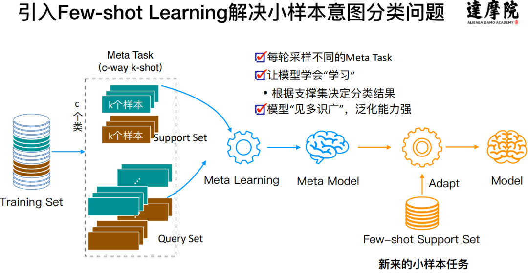
- meta training 阶段,将数据集分解为不同的 meta task,去学习类别变化的情况下模型的泛化能力
- meta testing 阶段,面对全新的类别,不需要变动已有的模型,就可以完成分类。
- Few-shot 的训练集中包含了很多的类别,每个类别中有多个样本。
- 在训练阶段,会在训练集中随机抽取 C 个类别,每个类别 K 个样本(总共 CK 个数据),构建一个 meta-task,作为模型的支撑集(support set)输入;
- 再从这 C 个类中剩余的数据中抽取一批(batch)样本作为模型的预测对象(batch set)。即要求模型从 C*K 个数据中学会如何区分这 C 个类别,这样的任务被称为 C-way K-shot 问题。
- 5 way 1 shot 示例
- 2-way 5-shot 示例

- meta training 阶段构建了一系列 meta-task 来让模型学习如何根据 support set 预测 batch set 中的样本的标签;
- meta testing 阶段的输入数据的形式与训练阶段一致(2-way 5-shot),但是会在全新的类别上构建 support set 和 batch。
- 训练过程中,每次训练(episode)都会采样得到不同 meta-task,所以总体来看,训练包含了不同的类别组合,这种机制使得模型学会不同 meta-task 中的共性部分,比如如何提取重要特征及比较样本相似等,忘掉 meta-task 中 task 相关部分。通过这种学习机制学到的模型,在面对新的未见过的 meta-task 时,也能较好地进行分类。

【2021-10-13】结合最新的Prompt Tuning的思想,PaddleNLP中集成了三大前沿FSL算法:
- EFL(Entailment as Few-Shot Learner),将 NLP Fine-tune任务统一转换为二分类的文本蕴含任务;
- PET(Pattern-Exploiting Training),通过人工构建模板,将分类任务转成完形填空任务;
- P-Tuning:自动构建模板,将模版的构建转化为连续参数优化问题。 使用小样本学习策略,仅仅32条样本即可在电商评论分类任务上取得87%的分类精度
数据集
- 图像
- MiniImage
- Omnigraffle
- 文本
- FewRel 数据集由Han等人在EMNLP 2018提出,是一个小样本关系分类数据集,包含64种关系用于训练,16种关系用于验证和20种关系用于测试,每种关系下包含700个样本。
- ARSC 数据集 由 Yu 等人在 NAACL 2018 提出,取自亚马逊多领域情感分类数据,该数据集包含 23 种亚马逊商品的评论数据,对于每一种商品,构建三个二分类任务,将其评论按分数分为 5、4、 2 三档,每一档视为一个二分类任务,则产生 233=69 个 task,然后取其中 12 个 task(43)作为测试集,其余 57 个 task 作为训练集。
- ODIC 数据集来自阿里巴巴对话工厂平台的线上日志,用户会向平台提交多种不同的对话任务,和多种不同的意图,但是每种意图只有极少数的标注数据,这形成了一个典型的 Few-shot Learning 任务,该数据集包含 216 个意图,其中 159 个用于训练,57 个用于测试。
Most popularly used datasets:
- Omniglot
- mini-ImageNet
- ILSVRC
- FGVC aircraft
- Caltech-UCSD Birds-200-2011 Check several other datasets by Google here.
方法
- 早期的 Few-shot Learning 算法研究多集中在图像领域,以 MiniImage 和 Omnigraffle 两个数据集为代表。
- 近年来,在自然语言处理领域也开始出现 Few-shot Learning 的数据集和模型,相比于图像,文本的语义中包含更多的变化和噪声
- Few-shot Learning 模型大致可分为三类:
- Mode Based:通过模型结构的设计快速在少量样本上更新参数,直接建立输入 x 和预测值 P 的映射函数
- Metric Based:通过度量 batch 中的样本和 support 中样本的距离,借助最近邻的思想完成分类
- Optimization Based:普通的梯度下降方法难以在 few-shot 场景下拟合,因此通过调整优化方法来完成小样本分类的任务
- Few shot learning中较为热门的方法大多是metric-based,即通过类别中少量样本计算得到该类别的表示,然后再用某种metric方法计算得到最终的分类结果。
- 【2021-7-8】阿里达摩院黎槟华,李永彬的基于小样本学习的对话意图识别
Model Based方法
- Santoro 等人提出使用记忆增强的方法来解决 Few-shot Learning 任务。基于记忆的神经网络方法早在 2001 年被证明可以用于 meta-learning。他们通过权重更新来调节 bias,并且通过学习将表达快速缓存到记忆中来调节输出。
- 然而,利用循环神经网络的内部记忆单元无法扩展到需要对大量新信息进行编码的新任务上。因此,需要让存储在记忆中的表达既要稳定又要是元素粒度访问的,前者是说当需要时就能可靠地访问,后者是说可选择性地访问相关的信息;另外,参数数量不能被内存的大小束缚。神经图灵机(NTMs)和记忆网络就符合这种必要条件。
- 文章基于神经网络图灵机(NTMs)的思想,因为 NTMs 能通过外部存储(external memory)进行短时记忆,并能通过缓慢权值更新来进行长时记忆,NTMs 可以学习将表达存入记忆的策略,并如何用这些表达来进行预测。由此,文章方法可以快速准确地预测那些只出现过一次的数据。
- 文章基于 LSTM 等 RNN 的模型,将数据看成序列来训练,在测试时输入新的类的样本进行分类。
- 具体地,在 t 时刻,模型输入 (xt,yt-1),也就是在当前时刻预测输入样本的类别,并在下一时刻给出真实的 label,并且添加了 external memory 存储上一次的 x 输入,这使得下一次输入后进行反向传播时,可以让 y (label) 和 x 建立联系,使得之后的 x 能够通过外部记忆获取相关图像进行比对来实现更好的预测。
- ▲ Memory Augmented Model
- Meta Network的快速泛化能力源自其“快速权重”的机制,在训练过程中产生的梯度被用来作为快速权重的生成。
- 模型包含一个 meta learner 和一个 base learner
- meta learner 用于学习 meta task 之间的泛化信息,并使用 memory 机制保存这种信息
- base learner 用于快速适应新的 task,并和 meta learner 交互产生预测输出。
Metric Based方法
- 如果在 Few-shot Learning 的任务中去训练普通的基于 cross-entropy 的神经网络分类器,那么几乎肯定是会过拟合,因为神经网络分类器中有数以万计的参数需要优化。
- 相反,很多非参数化的方法(最近邻、K-近邻、Kmeans)不需要优化参数,因此可以在 meta-learning 的框架下构造一种可以端到端训练的 few-shot 分类器。该方法是对样本间距离分布进行建模,使得同类样本靠近,异类样本远离。下面介绍相关的方法。
- 如图所示,孪生网络(Siamese Network)通过有监督的方式训练孪生网络来学习,然后重用网络所提取的特征进行 one/few-shot 学习。
- Siamese Network

- 知乎视频讲解:Few-Shot Learning - Siamese Network,使用triplet loss,同类相近,异类相远
- 双路神经网络
- 训练时,通过组合的方式构造不同的成对样本,输入网络进行训练,在最上层通过样本对的距离判断他们是否属于同一个类,并产生对应的概率分布。
- 预测时,孪生网络处理测试样本和支撑集之间每一个样本对,最终预测结果为支撑集上概率最高的类别。
- (1)相比孪生网络(连体网络),匹配网络(Match Network)为支撑集和 Batch 集构建不同的编码器,最终分类器的输出是支撑集样本和 query 之间预测值的加权求和。
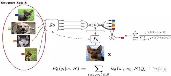
- 在不改变网络模型的前提下能对未知类别生成标签,其主要创新体现在建模过程和训练过程上。对于建模过程的创新,文章提出了基于 memory 和 attention 的 matching nets,使得可以快速学习。基于传统机器学习的一个原则,即训练和测试是要在同样条件下进行的,提出在训练的时候不断地让网络只看每一类的少量样本,这将和测试的过程是一致的。
- 支撑集样本 embedding 模型 g 能继续优化,并且支撑集样本应该可以用来修改测试样本的 embedding 模型 f。
- 这个可以通过如下两个方面来解决,即:
- 1)基于双向 LSTM 学习训练集的 embedding,使得每个支撑样本的 embedding 是其它训练样本的函数;
- 2)基于 attention-LSTM 来对测试样本 embedding,使得每个 Query 样本的 embedding 是支撑集 embedding 的函数。文章称其为 FCE (fully-conditional embedding)。
- (2)原型网络(Prototype Network)基于这样的想法:
- 每个类别都存在一个原型表达,该类的原型是 support set 在 embedding 空间中的均值。然后,分类问题变成在 embedding 空间中的最近邻。
- c1、c2、c3 分别是三个类别的均值中心(称 Prototype),将测试样本 x 进行 embedding 后,与这 3 个中心进行距离计算,从而获得 x 的类别。

- 文章采用在 Bregman 散度下的指数族分布的混合密度估计,文章在训练时采用相对测试时更多的类别数,即训练时每个 episodes 采用 20 个类(20 way),而测试对在 5 个类(5 way)中进行,其效果相对训练时也采用 5 way 的提升了 2.5 个百分点。
- 前面介绍的几个网络结构在最终的距离度量上都使用了固定的度量方式,如 cosine,欧式距离等,这种模型结构下所有的学习过程都发生在样本的 embedding 阶段。
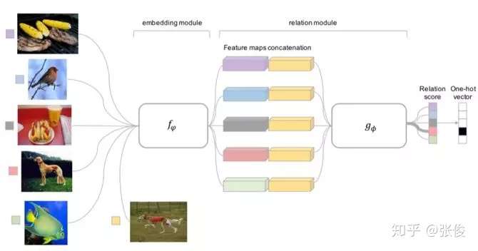
- (3)Relation Network
- Relation Network认为度量方式也是网络中非常重要的一环,需要对其进行建模,所以该网络不满足单一且固定的距离度量方式,而是训练一个网络来学习(例如 CNN)距离的度量方式,在 loss 方面也有所改变,考虑到 relation network 更多的关注 relation score,更像一种回归,而非 0/1 分类,所以使用了 MSE 取代了 cross-entropy。
Optimization Based方法
- Ravi 等人 [7] 研究了在少量数据下,基于梯度的优化算法失败的原因,即无法直接用于 meta learning。
- 首先,这些梯度优化算法包括 momentum, adagrad, adadelta, ADAM 等,无法在几步内完成优化,特别是在非凸的问题上,多种超参的选取无法保证收敛的速度。
- 其次,不同任务分别随机初始化会影响任务收敛到好的解上。虽然 fine tune 这种迁移学习能缓解这个问题,但当新数据相对原始数据偏差比较大时,迁移学习的性能会大大下降。我们需要一个系统的学习通用初始化,使得训练从一个好的点开始,它和迁移学习不同的是,它能保证该初始化能让 finetune 从一个好的点开始。
- 文章学习的是一个模型参数的更新函数或更新规则。它不是在多轮的 episodes 学习一个单模型,而是在每个 episode 学习特定的模型。
- 学习基于梯度下降的参数更新算法,采用 LSTM 表达 meta learner,用其状态表达目标分类器的参数的更新,最终学会如何在新的分类任务上,对分类器网络(learner)进行初始化和参数更新。这个优化算法同时考虑一个任务的短时知识和跨多个任务的长时知识。
- 文章设定目标为通过少量的迭代步骤捕获优化算法的泛化能力,由此 meta learner 可以训练让 learner 在每个任务上收敛到一个好的解。另外,通过捕获所有任务之前共享的基础知识,进而更好地初始化 learner。
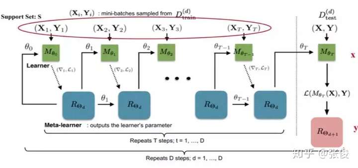
- 以训练 miniImage 数据集为例,训练过程中,从训练集(64 个类,每类 600 个样本)中随机采样 5 个类,每个类 5 个样本,构成支撑集,去学习 learner;然后从训练集的样本(采出的 5 个类,每类剩下的样本)中采样构成 Batch 集,集合中每类有 15 个样本,用来获得 learner 的 loss,去学习 meta leaner。
- 测试时的流程一样,从测试集(16 个类,每类 600 个样本)中随机采样 5 个类,每个类 5 个样本,构成支撑集 Support Set,去学习 learner;然后从测试集剩余的样本(采出的 5 个类,每类剩下的样本)中采样构成 Batch 集,集合中每类有 15 个样本,用来获得 learner 的参数,进而得到预测的类别概率。这两个过程分别如图 8 中虚线左侧和右侧。
- meta learner 的目标是在各种不同的学习任务上学出一个模型,使得可以仅用少量的样本就能解决一些新的学习任务。这种任务的挑战是模型需要结合之前的经验和当前新任务的少量样本信息,并避免在新数据上过拟合。
- Finn [8] 提出的方法使得可以在小量样本上,用少量的迭代步骤就可以获得较好的泛化性能,而且模型是容易 fine-tine 的。而且这个方法无需关心模型的形式,也不需要为 meta learning 增加新的参数,直接用梯度下降来训练 learner。
- 文章的核心思想是学习模型的初始化参数使得在一步或几步迭代后在新任务上的精度最大化。它学的不是模型参数的更新函数或是规则,它不局限于参数的规模和模型架构(比如用 RNN 或 siamese)。它本质上也是学习一个好的特征使得可以适合很多任务(包括分类、回归、增强学习),并通过 fine-tune 来获得好的效果。
- 文章提出的方法,可以学习任意标准模型的参数,并让该模型能快速适配。他们认为,一些中间表达更加适合迁移,比如神经网络的内部特征。因此面向泛化性的表达是有益的。因为我们会基于梯度下降策略在新的任务上进行 finetune,所以目标是学习这样一个模型,它能对新的任务从之前任务上快速地进行梯度下降,而不会过拟合。事实上,是要找到一些对任务变化敏感的参数,使得当改变梯度方向,小的参数改动也会产生较大的 loss。
案例
- 【2021-2-22】达摩院Conversational AI研究进展及应用
- 任务型对话引擎Dialog Studio和表格型问答引擎TableQA的核心技术研究进行介绍:
- 语言理解:如何系统解决低资源问题
- 低资源小样本问题
- 冷启动的场景下,统计45个POC机器人的数据,平均每个意图下的训练样本不到6条,是一个典型的小样本学习问题。
- 在脱离了冷启动阶段进入规模化阶段之后,小样本问题依然存在,比如对浙江省11个地市的12345热线机器人数据进行分析,在将近900个意图中,有42%的中长尾意图的训练样本少于10条,这仍然是一个典型的小样本学习问题。

- 解决方案:引入Few-shot Learning系统解决小样本问题;本质是一个迁移学习:迁移学习的方式能够最大化平台方积累数据的优势。即插即用的算法:在应用的时候不需要训练,可以灵活地增添新的数据,这对toB场景非常友好;
- 达摩院Conversational AI团队提出了一个Encoder-Induction-Relation的三层Few-shot learning Framework
- 无论是小孩子还是大人,从小样本中进行学习的时候,主要依靠的是两种强大的能力,归纳能力和记忆能力
- 达摩院提出了Dynamic Memory Induction Networks的动态记忆机制(发表于ACL2020)
- 低资源小样本问题
- 语言理解:如何系统解决低资源问题
- 任务型对话引擎Dialog Studio和表格型问答引擎TableQA的核心技术研究进行介绍:
Meta-Learning 元学习
- Meta learning
- 元学习的核心想法是先学习一个先验知识(prior),这个先验知识对解决 few-shot learning 问题特别有帮助。
- Meta-learning 中有 task 的概念,比如5-way 1-shot 问题就是一个 task,先学习很多很多这样的 task,然后再来解决这个新的 task 。重要的一点,这是一个新的 task。分类问题中,这个新的 task 中的类别是之前我们学习过的 task 中没有见过的! 在 Meta-learning 中之前学习的 task 我们称为 meta-training task,遇到的新的 task 称为 meta-testing task。因为每一个 task 都有自己的训练集和测试集,因此为了不引起混淆,我们把 task 内部的训练集和测试集一般称为 support set 和 query set
- Meta-learning 方法的分类标准有很多,为解决过拟合问题,有下面常见的3种方法
- 学习微调 (Learning to Fine-Tune)
- 基于 RNN 的记忆 (RNN Memory Based)
- 度量学习 (Metric Learning)
- 参考文章《Learning to Compare: Relation Network for Few-Shot Learning》
- 学习微调 (Learning to Fine-Tune)
- MAML(《Model-Agnostic Meta-Learning for Fast Adaptation of Deep Networks》) 是这类方法的范例之一。MAML 的思想是学习一个 初始化参数 (initialization parameter),这个初始化参数在遇到新的问题时,只需要使用少量的样本 (few-shot learning) 进行几步梯度下降就可以取得很好地效果( 参见后续博客 )。另一个典型是《Optimization as a Model for Few-Shot Learning》,他不仅关注于初始化,还训练了一个基于 LSTM 的优化器 (optimizer) 来帮助微调( 参见后续博客 )。
- 基于 RNN 的记忆 (RNN Memory Based)
- 最直观的方法,使用基于 RNN 的技术记忆先前 task 中的表示等,这种表示将有助于学习新的 task。可参考《Meta networks》和 《Meta-learning with memory-augmented neural networks.》
- 度量学习 (Metric Learning)
- 主要可以参考《Learning a Similarity Metric Discriminatively, with Application to Face Verification.》,《Siamese neural networks for one-shot image recognition》,《Siamese neural networks for one-shot image recognition》,《Matching networks for one shot learning》,《Prototypical Networks for Few-shot Learning》,《Learning to Compare: Relation Network for Few-Shot Learning》。 - 核心思想:学习一个 embedding 函数,将输入空间(例如图片)映射到一个新的嵌入空间,在嵌入空间中有一个相似性度量来区分不同类。我们的先验知识就是这个 embedding 函数,在遇到新的 task 的时候,只将需要分类的样本点用这个 embedding 函数映射到嵌入空间里面,使用相似性度量比较进行分类。
- 方法简单比较
- 基于 RNN 的记忆 (RNN Memory Based) 有两个关键问题,一个是这种方法经常会加一个外部存储来记忆,另一个是对模型进行了限制 (RNN),这可能会在一定程度上阻碍其发展和应用。
- 学习微调 (Learning to Fine-Tune) 的方法需要在新的 task 上面进行微调,也正是由于需要新的 task 中 support set 中有样本来进行微调,目前我个人还没看到这种方法用于 zero-shot learning(参考 few-shot learning 问题的定义,可以得到 zero-shot learning的定义)的问题上,但是在《Model-Agnostic Meta-Learning for Fast Adaptation of Deep Networks》的作者 Chelsea Finn 的博士论文《Learning to Learn with Gradients》中给出了 MAML 的理论证明,并且获得了 2018 ACM 最佳博士论文奖,还有一点就是 MAML 可以用于强化学习,另外两种方法多用于分类问题。链接
- 度量学习 (Metric Learning),和学习微调 (Learning to Fine-Tune) 的方法一样不对模型进行任何限制,并且可以用于 zero-shot learning 问题。虽然效果比较理想但是现在好像多用于分类任务并且可能缺乏一些理论上的证明,比如相似性度量是基于余弦距离还是欧式距离亦或是其他?为什么是这个距离?(因为 embedding 函数是一个神经网络,可解释性差,导致无法很好解释新的 embedding 空间),虽然《Learning to Compare: Relation Network for Few-Shot Learning》中的 Relation Network 将两个需要比较的 embedding 又送到一个神经网络(而不是人为手动选择相似性度量)来计算相似性得分,但是同样缺乏很好地理论证明。
- 参考:Few-shot learning(少样本学习)和 Meta-learning(元学习)概述
Meta-learning, also known as “learning to learn”, intends to design models that can learn new skills or adapt to new environments rapidly with a few training examples. There are three common approaches: 1) learn an efficient distance metric (metric-based); 2) use (recurrent) network with external or internal memory (model-based); 3) optimize the model parameters explicitly for fast learning (optimization-based).
[Updated on 2019-10-01: thanks to Tianhao, we have this post translated in Chinese!]
A good machine learning model often requires training with a large number of samples. Humans, in contrast, learn new concepts and skills much faster and more efficiently. Kids who have seen cats and birds only a few times can quickly tell them apart. People who know how to ride a bike are likely to discover the way to ride a motorcycle fast with little or even no demonstration. Is it possible to design a machine learning model with similar properties — learning new concepts and skills fast with a few training examples? That’s essentially what meta-learning aims to solve.
We expect a good meta-learning model capable of well adapting or generalizing to new tasks and new environments that have never been encountered during training time. The adaptation process, essentially a mini learning session, happens during test but with a limited exposure to the new task configurations. Eventually, the adapted model can complete new tasks. This is why meta-learning is also known as learning to learn.
The tasks can be any well-defined family of machine learning problems: supervised learning, reinforcement learning, etc. For example, here are a couple concrete meta-learning tasks:
- A classifier trained on non-cat images can tell whether a given image contains a cat after seeing a handful of cat pictures.
- A game bot is able to quickly master a new game.
- A mini robot completes the desired task on an uphill surface during test even through it was only trained in a flat surface environment.
- TOC
Define the Meta-Learning Problem
In this post, we focus on the case when each desired task is a supervised learning problem like image classification. There is a lot of interesting literature on meta-learning with reinforcement learning problems (aka “Meta Reinforcement Learning”), but we would not cover them here.
A Simple View
A good meta-learning model should be trained over a variety of learning tasks and optimized for the best performance on a distribution of tasks, including potentially unseen tasks. Each task is associated with a dataset \(\mathcal{D}\), containing both feature vectors and true labels. The optimal model parameters are:
\[\theta^* = \arg\min_\theta \mathbb{E}_{\mathcal{D}\sim p(\mathcal{D})} [\mathcal{L}_\theta(\mathcal{D})]\]It looks very similar to a normal learning task, but one dataset is considered as one data sample.
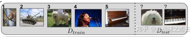
Few-shot classification is an instantiation of meta-learning in the field of supervised learning. The dataset \(\mathcal{D}\) is often split into two parts, a support set \(S\) for learning and a prediction set \(B\) for training or testing, \(\mathcal{D}=\langle S, B\rangle\). Often we consider a K-shot N-class classification task: the support set contains K labelled examples for each of N classes.
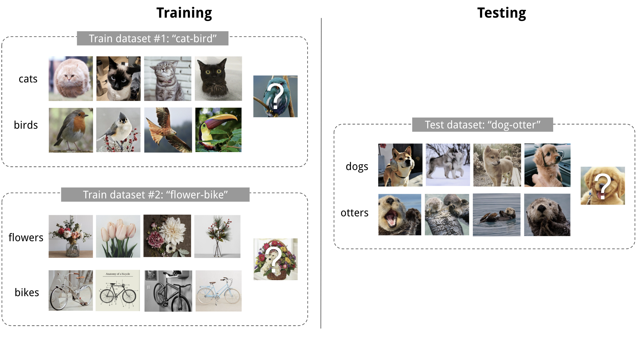
Fig. 1. An example of 4-shot 2-class image classification. (Image thumbnails are from Pinterest)
Training in the Same Way as Testing
A dataset \(\mathcal{D}\) contains pairs of feature vectors and labels, \(\mathcal{D} = \{(\mathbf{x}_i, y_i)\}\) and each label belongs to a known label set \(\mathcal{L}^\text{label}\). Let’s say, our classifier \(f_\theta\) with parameter \(\theta\) outputs a probability of a data point belonging to the class \(y\) given the feature vector \(\mathbf{x}\), \(P_\theta(y\vert\mathbf{x})\).
The optimal parameters should maximize the probability of true labels across multiple training batches \(B \subset \mathcal{D}\):
\[\begin{aligned} \theta^* &= {\arg\max}_{\theta} \mathbb{E}_{(\mathbf{x}, y)\in \mathcal{D}}[P_\theta(y \vert \mathbf{x})] &\\ \theta^* &= {\arg\max}_{\theta} \mathbb{E}_{B\subset \mathcal{D}}[\sum_{(\mathbf{x}, y)\in B}P_\theta(y \vert \mathbf{x})] & \scriptstyle{\text{; trained with mini-batches.}} \end{aligned}\]In few-shot classification, the goal is to reduce the prediction error on data samples with unknown labels given a small support set for “fast learning” (think of how “fine-tuning” works). To make the training process mimics what happens during inference, we would like to “fake” datasets with a subset of labels to avoid exposing all the labels to the model and modify the optimization procedure accordingly to encourage fast learning:
- Sample a subset of labels, \(L\subset\mathcal{L}^\text{label}\).
- Sample a support set \(S^L \subset \mathcal{D}\) and a training batch \(B^L \subset \mathcal{D}\). Both of them only contain data points with labels belonging to the sampled label set \(L\), \(y \in L, \forall (x, y) \in S^L, B^L\).
- The support set is part of the model input.
- The final optimization uses the mini-batch \(B^L\) to compute the loss and update the model parameters through backpropagation, in the same way as how we use it in the supervised learning.
You may consider each pair of sampled dataset \((S^L, B^L)\) as one data point. The model is trained such that it can generalize to other datasets. Symbols in red are added for meta-learning in addition to the supervised learning objective.
\[\theta = \arg\max_\theta \color{red}{E_{L\subset\mathcal{L}}[} E_{\color{red}{S^L \subset\mathcal{D}, }B^L \subset\mathcal{D}} [\sum_{(x, y)\in B^L} P_\theta(x, y\color{red}{, S^L})] \color{red}{]}\]The idea is to some extent similar to using a pre-trained model in image classification (ImageNet) or language modeling (big text corpora) when only a limited set of task-specific data samples are available. Meta-learning takes this idea one step further, rather than fine-tuning according to one down-steam task, it optimizes the model to be good at many, if not all.
Learner and Meta-Learner
Another popular view of meta-learning decomposes the model update into two stages:
- A classifier \(f_\theta\) is the “learner” model, trained for operating a given task;
- In the meantime, a optimizer \(g_\phi\) learns how to update the learner model’s parameters via the support set \(S\), \(\theta' = g_\phi(\theta, S)\).
Then in final optimization step, we need to update both \(\theta\) and \(\phi\) to maximize:
\[\mathbb{E}_{L\subset\mathcal{L}}[ \mathbb{E}_{S^L \subset\mathcal{D}, B^L \subset\mathcal{D}} [\sum_{(\mathbf{x}, y)\in B^L} P_{g_\phi(\theta, S^L)}(y \vert \mathbf{x})]]\]Common Approaches
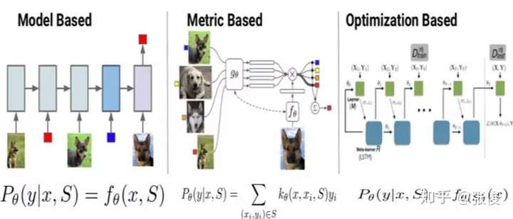
There are three common approaches to meta-learning: metric-based, model-based, and optimization-based. Oriol Vinyals has a nice summary in his talk at meta-learning symposium @ NIPS 2018:
| Model-based | Metric-based | Optimization-based | |
|---|---|---|---|
| Key idea | RNN; memory | Metric learning | Gradient descent |
| How \(P_\theta(y \vert \mathbf{x})\) is modeled? | \(f_\theta(\mathbf{x}, S)\) | \(\sum_{(\mathbf{x}_i, y_i) \in S} k_\theta(\mathbf{x}, \mathbf{x}_i)y_i\) (*) | \(P_{g_\phi(\theta, S^L)}(y \vert \mathbf{x})\) |
(*) \(k_\theta\) is a kernel function measuring the similarity between \(\mathbf{x}_i\) and \(\mathbf{x}\).
Next we are gonna review classic models in each approach.
Metric-Based
The core idea in metric-based meta-learning is similar to nearest neighbors algorithms (i.e., k-NN classificer and k-means clustering) and kernel density estimation. The predicted probability over a set of known labels \(y\) is a weighted sum of labels of support set samples. The weight is generated by a kernel function \(k_\theta\), measuring the similarity between two data samples.
\[P_\theta(y \vert \mathbf{x}, S) = \sum_{(\mathbf{x}_i, y_i) \in S} k_\theta(\mathbf{x}, \mathbf{x}_i)y_i\]To learn a good kernel is crucial to the success of a metric-based meta-learning model. Metric learning is well aligned with this intention, as it aims to learn a metric or distance function over objects. The notion of a good metric is problem-dependent. It should represent the relationship between inputs in the task space and facilitate problem solving.
All the models introduced below learn embedding vectors of input data explicitly and use them to design proper kernel functions.
Convolutional Siamese Neural Network
The Siamese Neural Network is composed of two twin networks and their outputs are jointly trained on top with a function to learn the relationship between pairs of input data samples. The twin networks are identical, sharing the same weights and network parameters. In other words, both refer to the same embedding network that learns an efficient embedding to reveal relationship between pairs of data points.
Koch, Zemel & Salakhutdinov (2015) proposed a method to use the siamese neural network to do one-shot image classification. First, the siamese network is trained for a verification task for telling whether two input images are in the same class. It outputs the probability of two images belonging to the same class. Then, during test time, the siamese network processes all the image pairs between a test image and every image in the support set. The final prediction is the class of the support image with the highest probability.
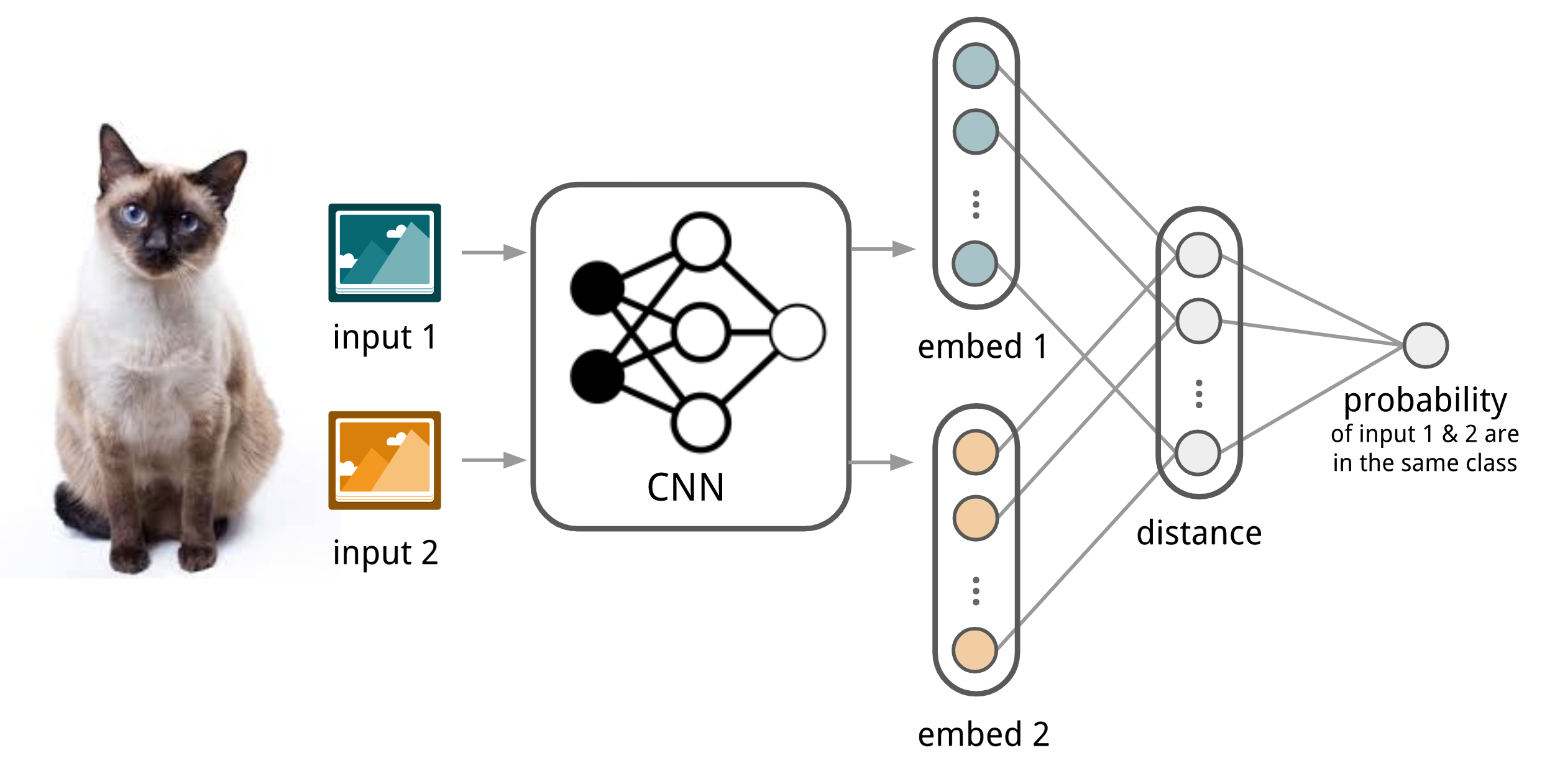
Fig. 2. The architecture of convolutional siamese neural network for few-show image classification.
- First, convolutional siamese network learns to encode two images into feature vectors via a embedding function \(f_\theta\) which contains a couple of convolutional layers.
- The L1-distance between two embeddings is \(\vert f_\theta(\mathbf{x}_i) - f_\theta(\mathbf{x}_j) \vert\).
- The distance is converted to a probability \(p\) by a linear feedforward layer and sigmoid. It is the probability of whether two images are drawn from the same class.
- Intuitively the loss is cross entropy because the label is binary.
Images in the training batch \(B\) can be augmented with distortion. Of course, you can replace the L1 distance with other distance metric, L2, cosine, etc. Just make sure they are differential and then everything else works the same.
Given a support set \(S\) and a test image \(\mathbf{x}\), the final predicted class is:
\[\hat{c}_S(\mathbf{x}) = c(\arg\max_{\mathbf{x}_i \in S} P(\mathbf{x}, \mathbf{x}_i))\]where \(c(\mathbf{x})\) is the class label of an image \(\mathbf{x}\) and \(\hat{c}(.)\) is the predicted label.
The assumption is that the learned embedding can be generalized to be useful for measuring the distance between images of unknown categories. This is the same assumption behind transfer learning via the adoption of a pre-trained model; for example, the convolutional features learned in the model pre-trained with ImageNet are expected to help other image tasks. However, the benefit of a pre-trained model decreases when the new task diverges from the original task that the model was trained on.
Matching Networks
The task of Matching Networks (Vinyals et al., 2016) is to learn a classifier \(c_S\) for any given (small) support set \(S=\{x_i, y_i\}_{i=1}^k\) (k-shot classification). This classifier defines a probability distribution over output labels \(y\) given a test example \(\mathbf{x}\). Similar to other metric-based models, the classifier output is defined as a sum of labels of support samples weighted by attention kernel \(a(\mathbf{x}, \mathbf{x}_i)\) - which should be proportional to the similarity between \(\mathbf{x}\) and \(\mathbf{x}_i\).
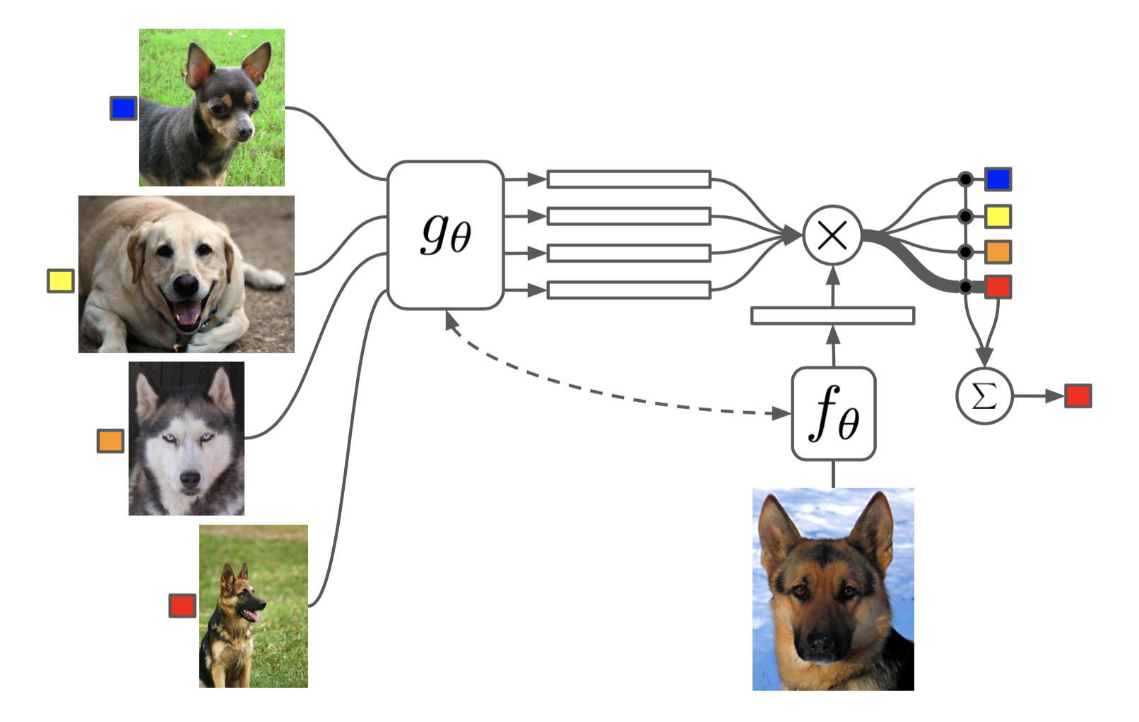
Fig. 3. The architecture of Matching Networks. (Image source: original paper)
\[c_S(\mathbf{x}) = P(y \vert \mathbf{x}, S) = \sum_{i=1}^k a(\mathbf{x}, \mathbf{x}_i) y_i \text{, where }S=\{(\mathbf{x}_i, y_i)\}_{i=1}^k\]The attention kernel depends on two embedding functions, \(f\) and \(g\), for encoding the test sample and the support set samples respectively. The attention weight between two data points is the cosine similarity, \(\text{cosine}(.)\), between their embedding vectors, normalized by softmax:
\[a(\mathbf{x}, \mathbf{x}_i) = \frac{\exp(\text{cosine}(f(\mathbf{x}), g(\mathbf{x}_i))}{\sum_{j=1}^k\exp(\text{cosine}(f(\mathbf{x}), g(\mathbf{x}_j))}\]Simple Embedding
In the simple version, an embedding function is a neural network with a single data sample as input. Potentially we can set \(f=g\).
Full Context Embeddings
The embedding vectors are critical inputs for building a good classifier. Taking a single data point as input might not be enough to efficiently gauge the entire feature space. Therefore, the Matching Network model further proposed to enhance the embedding functions by taking as input the whole support set \(S\) in addition to the original input, so that the learned embedding can be adjusted based on the relationship with other support samples.
- \(g_\theta(\mathbf{x}_i, S)\) uses a bidirectional LSTM to encode \(\mathbf{x}_i\) in the context of the entire support set \(S\).
- \(f_\theta(\mathbf{x}, S)\) encodes the test sample \(\mathbf{x}\) visa an LSTM with read attention over the support set \(S\).
- First the test sample goes through a simple neural network, such as a CNN, to extract basic features, \(f'(\mathbf{x})\).
- Then an LSTM is trained with a read attention vector over the support set as part of the hidden state:
\(\begin{aligned} \hat{\mathbf{h}}_t, \mathbf{c}_t &= \text{LSTM}(f'(\mathbf{x}), [\mathbf{h}_{t-1}, \mathbf{r}_{t-1}], \mathbf{c}_{t-1}) \\ \mathbf{h}_t &= \hat{\mathbf{h}}_t + f'(\mathbf{x}) \\ \mathbf{r}_{t-1} &= \sum_{i=1}^k a(\mathbf{h}_{t-1}, g(\mathbf{x}_i)) g(\mathbf{x}_i) \\ a(\mathbf{h}_{t-1}, g(\mathbf{x}_i)) &= \text{softmax}(\mathbf{h}_{t-1}^\top g(\mathbf{x}_i)) = \frac{\exp(\mathbf{h}_{t-1}^\top g(\mathbf{x}_i))}{\sum_{j=1}^k \exp(\mathbf{h}_{t-1}^\top g(\mathbf{x}_j))} \end{aligned}\) - Eventually \(f(\mathbf{x}, S)=\mathbf{h}_K\) if we do K steps of “read”.
This embedding method is called “Full Contextual Embeddings (FCE)”. Interestingly it does help improve the performance on a hard task (few-shot classification on mini ImageNet), but makes no difference on a simple task (Omniglot).
The training process in Matching Networks is designed to match inference at test time, see the details in the earlier section. It is worthy of mentioning that the Matching Networks paper refined the idea that training and testing conditions should match.
\[\theta^* = \arg\max_\theta \mathbb{E}_{L\subset\mathcal{L}}[ \mathbb{E}_{S^L \subset\mathcal{D}, B^L \subset\mathcal{D}} [\sum_{(\mathbf{x}, y)\in B^L} P_\theta(y\vert\mathbf{x}, S^L)]]\]Relation Network
Relation Network (RN) (Sung et al., 2018) is similar to siamese network but with a few differences:
- The relationship is not captured by a simple L1 distance in the feature space, but predicted by a CNN classifier \(g_\phi\). The relation score between a pair of inputs, \(\mathbf{x}_i\) and \(\mathbf{x}_j\), is \(r_{ij} = g_\phi([\mathbf{x}_i, \mathbf{x}_j])\) where \([.,.]\) is concatenation.
- The objective function is MSE loss instead of cross-entropy, because conceptually RN focuses more on predicting relation scores which is more like regression, rather than binary classification, \(\mathcal{L}(B) = \sum_{(\mathbf{x}_i, \mathbf{x}_j, y_i, y_j)\in B} (r_{ij} - \mathbf{1}_{y_i=y_j})^2\).
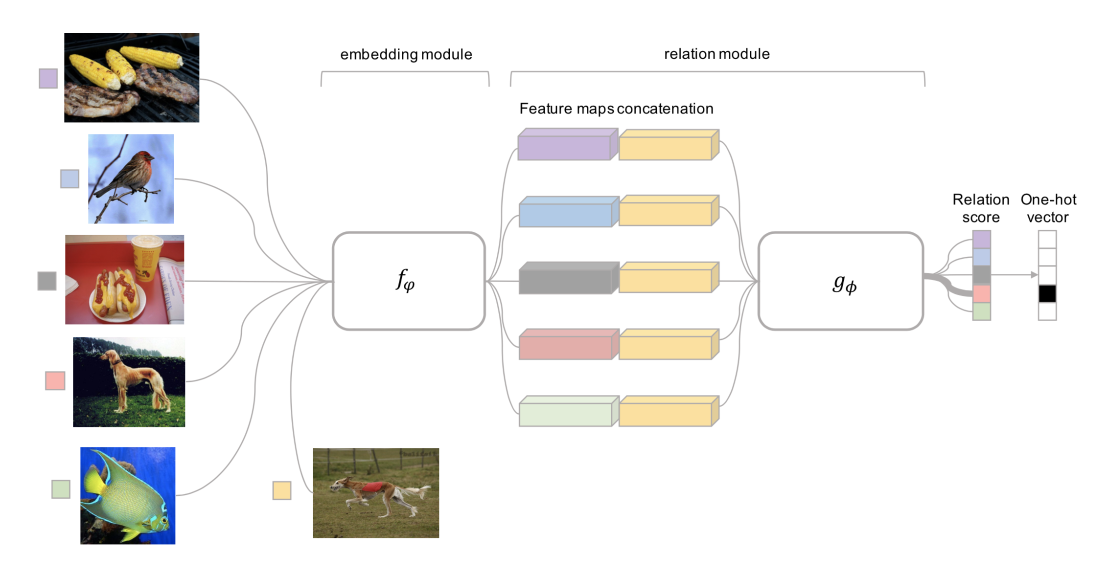
Fig. 4. Relation Network architecture for a 5-way 1-shot problem with one query example. (Image source: original paper)
(Note: There is another Relation Network for relational reasoning, proposed by DeepMind. Don’t get confused.)
Prototypical Networks
Prototypical Networks (Snell, Swersky & Zemel, 2017) use an embedding function \(f_\theta\) to encode each input into a \(M\)-dimensional feature vector. A prototype feature vector is defined for every class \(c \in \mathcal{C}\), as the mean vector of the embedded support data samples in this class.
\[\mathbf{v}_c = \frac{1}{|S_c|} \sum_{(\mathbf{x}_i, y_i) \in S_c} f_\theta(\mathbf{x}_i)\]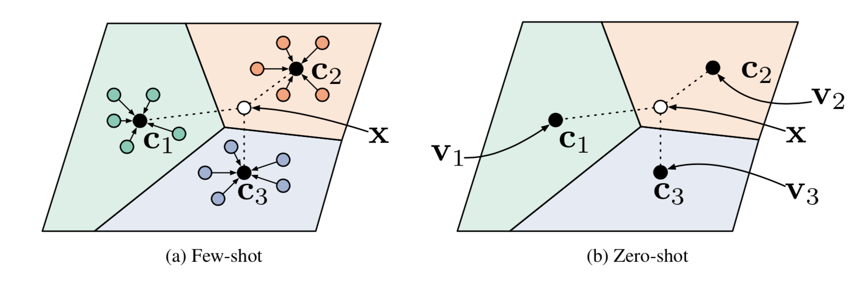
Fig. 5. Prototypical networks in the few-shot and zero-shot scenarios. (Image source: original paper)
The distribution over classes for a given test input \(\mathbf{x}\) is a softmax over the inverse of distances between the test data embedding and prototype vectors.
\[P(y=c\vert\mathbf{x})=\text{softmax}(-d_\varphi(f_\theta(\mathbf{x}), \mathbf{v}_c)) = \frac{\exp(-d_\varphi(f_\theta(\mathbf{x}), \mathbf{v}_c))}{\sum_{c' \in \mathcal{C}}\exp(-d_\varphi(f_\theta(\mathbf{x}), \mathbf{v}_{c'}))}\]where \(d_\varphi\) can be any distance function as long as \(\varphi\) is differentiable. In the paper, they used the squared euclidean distance.
The loss function is the negative log-likelihood: \(\mathcal{L}(\theta) = -\log P_\theta(y=c\vert\mathbf{x})\).
Model-Based
Model-based meta-learning models make no assumption on the form of \(P_\theta(y\vert\mathbf{x})\). Rather it depends on a model designed specifically for fast learning — a model that updates its parameters rapidly with a few training steps. This rapid parameter update can be achieved by its internal architecture or controlled by another meta-learner model.
Memory-Augmented Neural Networks
A family of model architectures use external memory storage to facilitate the learning process of neural networks, including Neural Turing Machines and Memory Networks. With an explicit storage buffer, it is easier for the network to rapidly incorporate new information and not to forget in the future. Such a model is known as MANN, short for “Memory-Augmented Neural Network”. Note that recurrent neural networks with only internal memory such as vanilla RNN or LSTM are not MANNs.
Because MANN is expected to encode new information fast and thus to adapt to new tasks after only a few samples, it fits well for meta-learning. Taking the Neural Turing Machine (NTM) as the base model, Santoro et al. (2016) proposed a set of modifications on the training setup and the memory retrieval mechanisms (or “addressing mechanisms”, deciding how to assign attention weights to memory vectors). Please go through the NTM section in my other post first if you are not familiar with this matter before reading forward.
As a quick recap, NTM couples a controller neural network with external memory storage. The controller learns to read and write memory rows by soft attention, while the memory serves as a knowledge repository. The attention weights are generated by its addressing mechanism: content-based + location based.
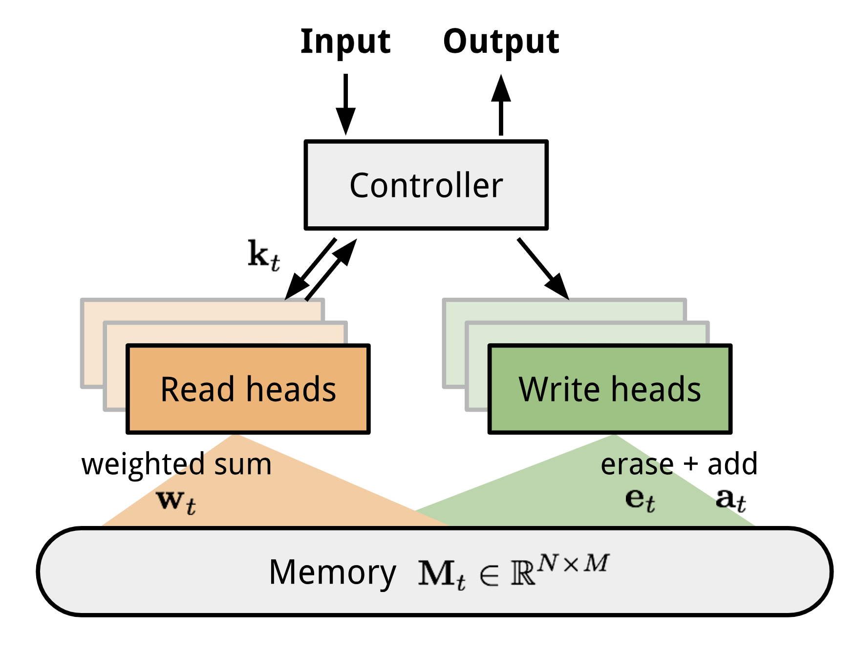
Fig. 6. The architecture of Neural Turing Machine (NTM). The memory at time t, \(\mathbf{M}_t\) is a matrix of size \(N \times M\), containing N vector rows and each has M dimensions.
MANN for Meta-Learning
To use MANN for meta-learning tasks, we need to train it in a way that the memory can encode and capture information of new tasks fast and, in the meantime, any stored representation is easily and stably accessible.
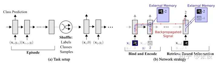
The training described in Santoro et al., 2016 happens in an interesting way so that the memory is forced to hold information for longer until the appropriate labels are presented later. In each training episode, the truth label \(y_t\) is presented with one step offset, \((\mathbf{x}_{t+1}, y_t)\): it is the true label for the input at the previous time step t, but presented as part of the input at time step t+1.
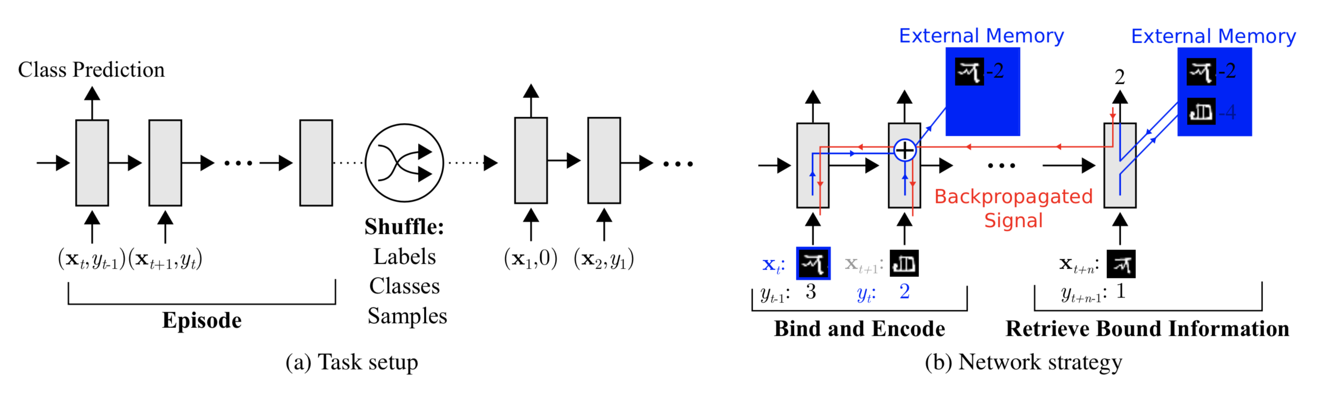
Fig. 7. Task setup in MANN for meta-learning (Image source: original paper).
In this way, MANN is motivated to memorize the information of a new dataset, because the memory has to hold the current input until the label is present later and then retrieve the old information to make a prediction accordingly.
Next let us see how the memory is updated for efficient information retrieval and storage.
Addressing Mechanism for Meta-Learning
Aside from the training process, a new pure content-based addressing mechanism is utilized to make the model better suitable for meta-learning.
» How to read from memory?
The read attention is constructed purely based on the content similarity.
First, a key feature vector \(\mathbf{k}_t\) is produced at the time step t by the controller as a function of the input \(\mathbf{x}\). Similar to NTM, a read weighting vector \(\mathbf{w}_t^r\) of N elements is computed as the cosine similarity between the key vector and every memory vector row, normalized by softmax. The read vector \(\mathbf{r}_t\) is a sum of memory records weighted by such weightings:
\[\mathbf{r}_i = \sum_{i=1}^N w_t^r(i)\mathbf{M}_t(i) \text{, where } w_t^r(i) = \text{softmax}(\frac{\mathbf{k}_t \cdot \mathbf{M}_t(i)}{\|\mathbf{k}_t\| \cdot \|\mathbf{M}_t(i)\|})\]where \(M_t\) is the memory matrix at time t and \(M_t(i)\) is the i-th row in this matrix.
» How to write into memory?
The addressing mechanism for writing newly received information into memory operates a lot like the cache replacement policy. The Least Recently Used Access (LRUA) writer is designed for MANN to better work in the scenario of meta-learning. A LRUA write head prefers to write new content to either the least used memory location or the most recently used memory location.
- Rarely used locations: so that we can preserve frequently used information (see LFU);
- The last used location: the motivation is that once a piece of information is retrieved once, it probably won’t be called again for a while (see MRU).
There are many cache replacement algorithms and each of them could potentially replace the design here with better performance in different use cases. Furthermore, it would be a good idea to learn the memory usage pattern and addressing strategies rather than arbitrarily set it.
The preference of LRUA is carried out in a way that everything is differentiable:
- The usage weight \(\mathbf{w}^u_t\) at time t is a sum of current read and write vectors, in addition to the decayed last usage weight, \(\gamma \mathbf{w}^u_{t-1}\), where \(\gamma\) is a decay factor.
- The write vector is an interpolation between the previous read weight (prefer “the last used location”) and the previous least-used weight (prefer “rarely used location”). The interpolation parameter is the sigmoid of a hyperparameter \(\alpha\).
- The least-used weight \(\mathbf{w}^{lu}\) is scaled according to usage weights \(\mathbf{w}_t^u\), in which any dimension remains at 1 if smaller than the n-th smallest element in the vector and 0 otherwise.
Finally, after the least used memory location, indicated by \(\mathbf{w}_t^{lu}\), is set to zero, every memory row is updated:
\[\mathbf{M}_t(i) = \mathbf{M}_{t-1}(i) + w_t^w(i)\mathbf{k}_t, \forall i\]Meta Networks
Meta Networks (Munkhdalai & Yu, 2017), short for MetaNet, is a meta-learning model with architecture and training process designed for rapid generalization across tasks.
Fast Weights
The rapid generalization of MetaNet relies on “fast weights”. There are a handful of papers on this topic, but I haven’t read all of them in detail and I failed to find a very concrete definition, only a vague agreement on the concept. Normally weights in the neural networks are updated by stochastic gradient descent in an objective function and this process is known to be slow. One faster way to learn is to utilize one neural network to predict the parameters of another neural network and the generated weights are called fast weights. In comparison, the ordinary SGD-based weights are named slow weights.
In MetaNet, loss gradients are used as meta information to populate models that learn fast weights. Slow and fast weights are combined to make predictions in neural networks.
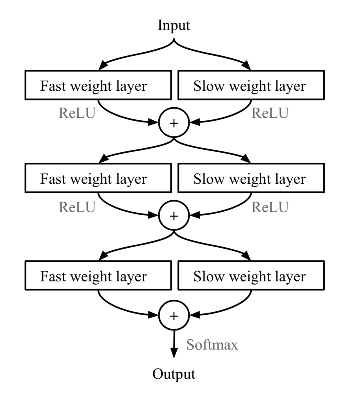
Fig. 8. Combining slow and fast weights in a MLP. \(\bigoplus\) is element-wise sum. (Image source: original paper).
Model Components
Disclaimer: Below you will find my annotations are different from those in the paper. imo, the paper is poorly written, but the idea is still interesting. So I’m presenting the idea in my own language.
Key components of MetaNet are:
- An embedding function \(f_\theta\), parameterized by \(\theta\), encodes raw inputs into feature vectors. Similar to Siamese Neural Network, these embeddings are trained to be useful for telling whether two inputs are of the same class (verification task).
- A base learner model \(g_\phi\), parameterized by weights \(\phi\), completes the actual learning task.
If we stop here, it looks just like Relation Network. MetaNet, in addition, explicitly models the fast weights of both functions and then aggregates them back into the model (See Fig. 8).
Therefore we need additional two functions to output fast weights for \(f\) and \(g\) respectively.
- \(F_w\): a LSTM parameterized by \(w\) for learning fast weights \(\theta^+\) of the embedding function \(f\). It takes as input gradients of \(f\)’s embedding loss for verification task.
- \(G_v\): a neural network parameterized by \(v\) learning fast weights \(\phi^+\) for the base learner \(g\) from its loss gradients. In MetaNet, the learner’s loss gradients are viewed as the meta information of the task.
Ok, now let’s see how meta networks are trained. The training data contains multiple pairs of datasets: a support set \(S=\{\mathbf{x}'_i, y'_i\}_{i=1}^K\) and a test set \(U=\{\mathbf{x}_i, y_i\}_{i=1}^L\). Recall that we have four networks and four sets of model parameters to learn, \((\theta, \phi, w, v)\).
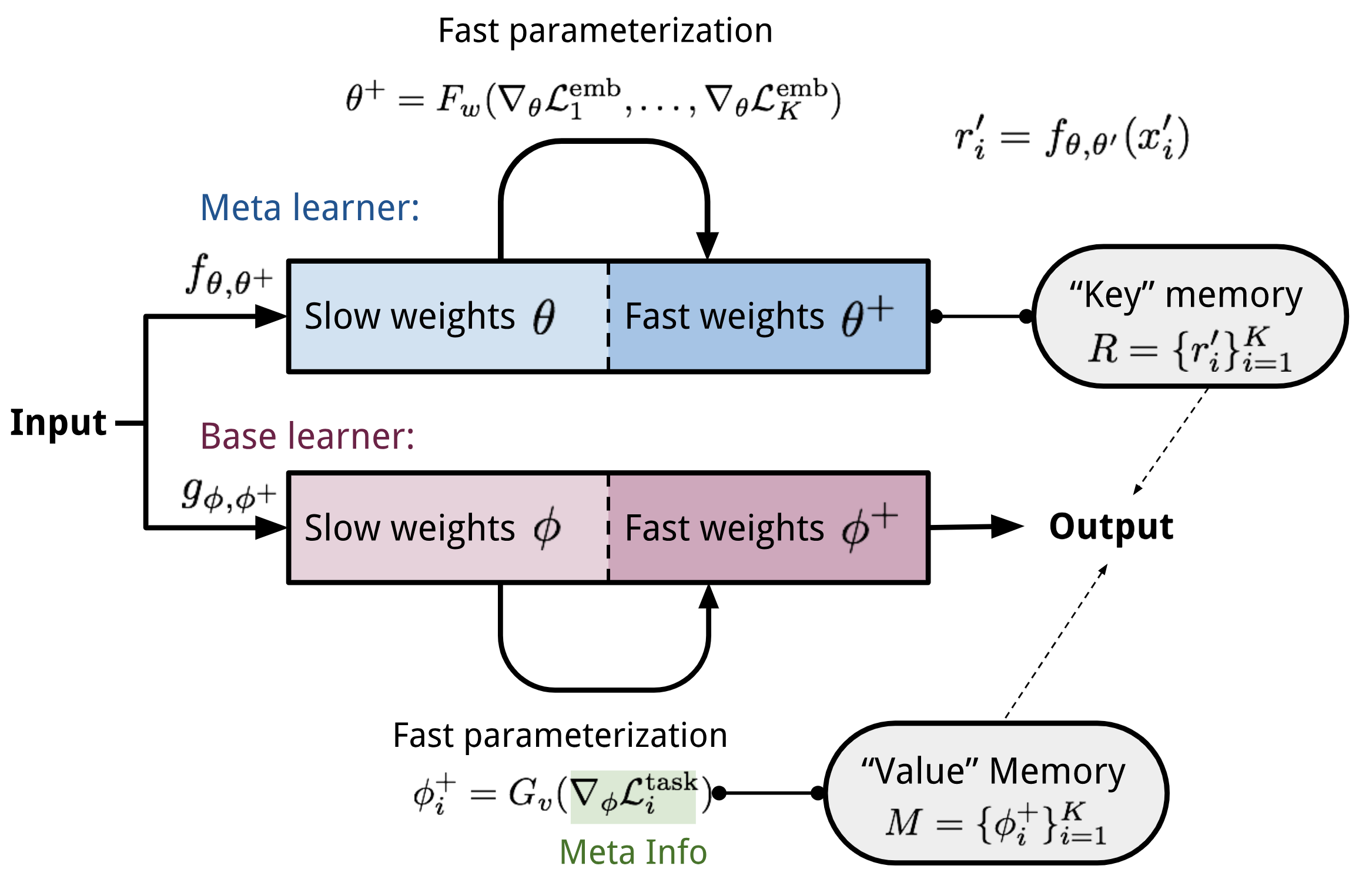
Fig.9. The MetaNet architecture.
Training Process
- Sample a random pair of inputs at each time step t from the support set \(S\), \((\mathbf{x}'_i, y'_i)\) and \((\mathbf{x}'_j, y_j)\). Let \(\mathbf{x}_{(t,1)}=\mathbf{x}'_i\) and \(\mathbf{x}_{(t,2)}=\mathbf{x}'_j\).
for \(t = 1, \dots, K\):- a. Compute a loss for representation learning; i.e., cross entropy for the verification task:
\(\mathcal{L}^\text{emb}_t = \mathbf{1}_{y'_i=y'_j} \log P_t + (1 - \mathbf{1}_{y'_i=y'_j})\log(1 - P_t)\text{, where }P_t = \sigma(\mathbf{W}\vert f_\theta(\mathbf{x}_{(t,1)}) - f_\theta(\mathbf{x}_{(t,2)})\vert)\)
- a. Compute a loss for representation learning; i.e., cross entropy for the verification task:
- Compute the task-level fast weights: \(\theta^+ = F_w(\nabla_\theta \mathcal{L}^\text{emb}_1, \dots, \mathcal{L}^\text{emb}_T)\)
- Next go through examples in the support set \(S\) and compute the example-level fast weights. Meanwhile, update the memory with learned representations.
for \(i=1, \dots, K\):- a. The base learner outputs a probability distribution: \(P(\hat{y}_i \vert \mathbf{x}_i) = g_\phi(\mathbf{x}_i)\) and the loss can be cross-entropy or MSE: \(\mathcal{L}^\text{task}_i = y'_i \log g_\phi(\mathbf{x}'_i) + (1- y'_i) \log (1 - g_\phi(\mathbf{x}'_i))\)
- b. Extract meta information (loss gradients) of the task and compute the example-level fast weights:
\(\phi_i^+ = G_v(\nabla_\phi\mathcal{L}^\text{task}_i)\)
- Then store \(\phi^+_i\) into \(i\)-th location of the “value” memory \(\mathbf{M}\).
- Then store \(\phi^+_i\) into \(i\)-th location of the “value” memory \(\mathbf{M}\).
- d. Encode the support sample into a task-specific input representation using both slow and fast weights: \(r'_i = f_{\theta, \theta^+}(\mathbf{x}'_i)\)
- Then store \(r'_i\) into \(i\)-th location of the “key” memory \(\mathbf{R}\).
- Finally it is the time to construct the training loss using the test set \(U=\{\mathbf{x}_i, y_i\}_{i=1}^L\).
Starts with \(\mathcal{L}_\text{train}=0\):
for \(j=1, \dots, L\):- a. Encode the test sample into a task-specific input representation: \(r_j = f_{\theta, \theta^+}(\mathbf{x}_j)\)
- b. The fast weights are computed by attending to representations of support set samples in memory \(\mathbf{R}\). The attention function is of your choice. Here MetaNet uses cosine similarity:
\(\begin{aligned} a_j &= \text{cosine}(\mathbf{R}, r_j) = [\frac{r'_1\cdot r_j}{\|r'_1\|\cdot\|r_j\|}, \dots, \frac{r'_N\cdot r_j}{\|r'_N\|\cdot\|r_j\|}]\\ \phi^+_j &= \text{softmax}(a_j)^\top \mathbf{M} \end{aligned}\) - c. Update the training loss: \(\mathcal{L}_\text{train} \leftarrow \mathcal{L}_\text{train} + \mathcal{L}^\text{task}(g_{\phi, \phi^+}(\mathbf{x}_i), y_i)\)
- Update all the parameters \((\theta, \phi, w, v)\) using \(\mathcal{L}_\text{train}\).
Optimization-Based
Deep learning models learn through backpropagation of gradients. However, the gradient-based optimization is neither designed to cope with a small number of training samples, nor to converge within a small number of optimization steps. Is there a way to adjust the optimization algorithm so that the model can be good at learning with a few examples? This is what optimization-based approach meta-learning algorithms intend for.
LSTM Meta-Learner
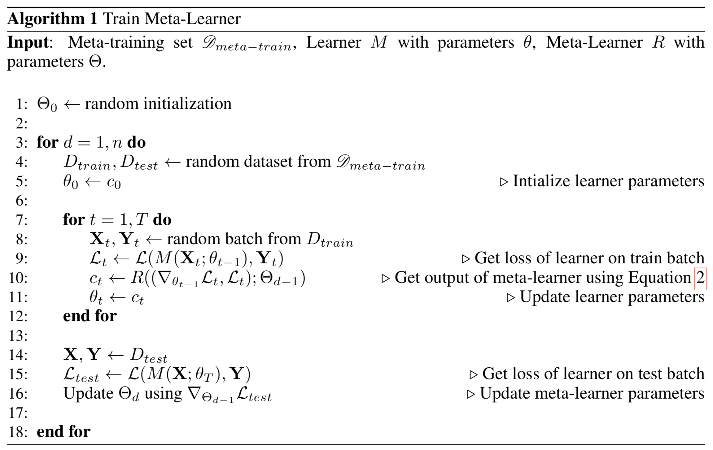
The optimization algorithm can be explicitly modeled. Ravi & Larochelle (2017) did so and named it “meta-learner”, while the original model for handling the task is called “learner”. The goal of the meta-learner is to efficiently update the learner’s parameters using a small support set so that the learner can adapt to the new task quickly.
Let’s denote the learner model as \(M_\theta\) parameterized by \(\theta\), the meta-learner as \(R_\Theta\) with parameters \(\Theta\), and the loss function \(\mathcal{L}\).
Why LSTM?
The meta-learner is modeled as a LSTM, because:
- There is similarity between the gradient-based update in backpropagation and the cell-state update in LSTM.
- Knowing a history of gradients benefits the gradient update; think about how momentum works.
The update for the learner’s parameters at time step t with a learning rate \(\alpha_t\) is:
\[\theta_t = \theta_{t-1} - \alpha_t \nabla_{\theta_{t-1}}\mathcal{L}_t\]It has the same form as the cell state update in LSTM, if we set forget gate \(f_t=1\), input gate \(i_t = \alpha_t\), cell state \(c_t = \theta_t\), and new cell state \(\tilde{c}_t = -\nabla_{\theta_{t-1}}\mathcal{L}_t\):
\[\begin{aligned} c_t &= f_t \odot c_{t-1} + i_t \odot \tilde{c}_t\\ &= \theta_{t-1} - \alpha_t\nabla_{\theta_{t-1}}\mathcal{L}_t \end{aligned}\]While fixing \(f_t=1\) and \(i_t=\alpha_t\) might not be the optimal, both of them can be learnable and adaptable to different datasets.
\[\begin{aligned} f_t &= \sigma(\mathbf{W}_f \cdot [\nabla_{\theta_{t-1}}\mathcal{L}_t, \mathcal{L}_t, \theta_{t-1}, f_{t-1}] + \mathbf{b}_f) & \scriptstyle{\text{; how much to forget the old value of parameters.}}\\ i_t &= \sigma(\mathbf{W}_i \cdot [\nabla_{\theta_{t-1}}\mathcal{L}_t, \mathcal{L}_t, \theta_{t-1}, i_{t-1}] + \mathbf{b}_i) & \scriptstyle{\text{; corresponding to the learning rate at time step t.}}\\ \tilde{\theta}_t &= -\nabla_{\theta_{t-1}}\mathcal{L}_t &\\ \theta_t &= f_t \odot \theta_{t-1} + i_t \odot \tilde{\theta}_t &\\ \end{aligned}\]Model Setup
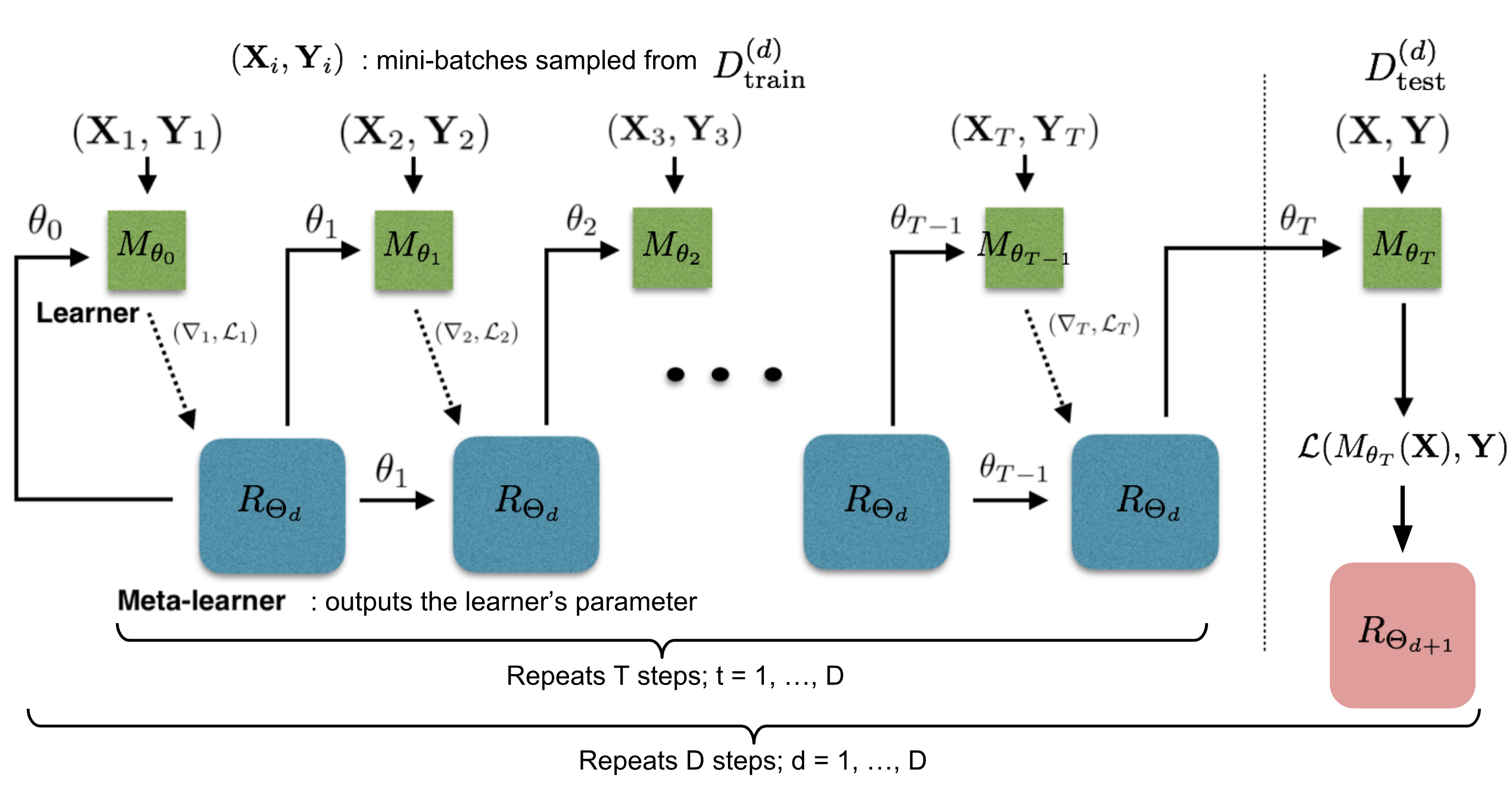
Fig.10. How the learner \(M_\theta\) and the meta-learner \(R_\Theta\) are trained. (Image source: original paper with more annotations)
The training process mimics what happens during test, since it has been proved to be beneficial in Matching Networks. During each training epoch, we first sample a dataset \(\mathcal{D} = (\mathcal{D}_\text{train}, \mathcal{D}_\text{test}) \in \hat{\mathcal{D}}_\text{meta-train}\) and then sample mini-batches out of \(\mathcal{D}_\text{train}\) to update \(\theta\) for \(T\) rounds. The final state of the learner parameter \(\theta_T\) is used to train the meta-learner on the test data \(\mathcal{D}_\text{test}\).
Two implementation details to pay extra attention to:
- How to compress the parameter space in LSTM meta-learner? As the meta-learner is modeling parameters of another neural network, it would have hundreds of thousands of variables to learn. Following the idea of sharing parameters across coordinates,
- To simplify the training process, the meta-learner assumes that the loss \(\mathcal{L}_t\) and the gradient \(\nabla_{\theta_{t-1}} \mathcal{L}_t\) are independent.
MAML
MAML, short for Model-Agnostic Meta-Learning (Finn, et al. 2017) is a fairly general optimization algorithm, compatible with any model that learns through gradient descent.
Let’s say our model is \(f_\theta\) with parameters \(\theta\). Given a task \(\tau_i\) and its associated dataset \((\mathcal{D}^{(i)}_\text{train}, \mathcal{D}^{(i)}_\text{test})\), we can update the model parameters by one or more gradient descent steps (the following example only contains one step):
\[\theta'_i = \theta - \alpha \nabla_\theta\mathcal{L}^{(0)}_{\tau_i}(f_\theta)\]where \(\mathcal{L}^{(0)}\) is the loss computed using the mini data batch with id (0).
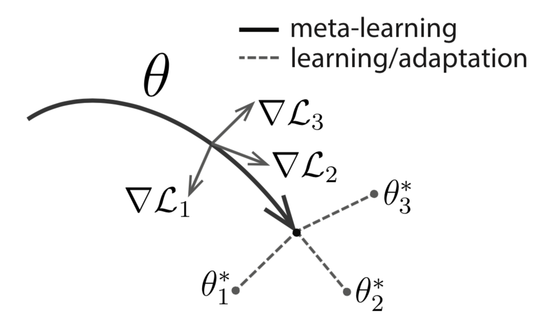
Fig. 11. Diagram of MAML. (Image source: original paper)
Well, the above formula only optimizes for one task. To achieve a good generalization across a variety of tasks, we would like to find the optimal \(\theta^*\) so that the task-specific fine-tuning is more efficient. Now, we sample a new data batch with id (1) for updating the meta-objective. The loss, denoted as \(\mathcal{L}^{(1)}\), depends on the mini batch (1). The superscripts in \(\mathcal{L}^{(0)}\) and \(\mathcal{L}^{(1)}\) only indicate different data batches, and they refer to the same loss objective for the same task.
\[\begin{aligned} \theta^* &= \arg\min_\theta \sum_{\tau_i \sim p(\tau)} \mathcal{L}_{\tau_i}^{(1)} (f_{\theta'_i}) = \arg\min_\theta \sum_{\tau_i \sim p(\tau)} \mathcal{L}_{\tau_i}^{(1)} (f_{\theta - \alpha\nabla_\theta \mathcal{L}_{\tau_i}^{(0)}(f_\theta)}) & \\ \theta &\leftarrow \theta - \beta \nabla_{\theta} \sum_{\tau_i \sim p(\tau)} \mathcal{L}_{\tau_i}^{(1)} (f_{\theta - \alpha\nabla_\theta \mathcal{L}_{\tau_i}^{(0)}(f_\theta)}) & \scriptstyle{\text{; updating rule}} \end{aligned}\]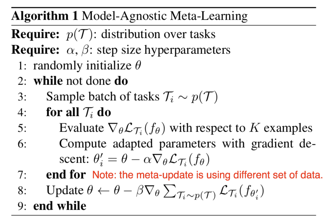
Fig. 12. The general form of MAML algorithm. (Image source: original paper)
First-Order MAML
The meta-optimization step above relies on second derivatives. To make the computation less expensive, a modified version of MAML omits second derivatives, resulting in a simplified and cheaper implementation, known as First-Order MAML (FOMAML).
Let’s consider the case of performing \(k\) inner gradient steps, \(k\geq1\). Starting with the initial model parameter \(\theta_\text{meta}\):
\[\begin{aligned} \theta_0 &= \theta_\text{meta}\\ \theta_1 &= \theta_0 - \alpha\nabla_\theta\mathcal{L}^{(0)}(\theta_0)\\ \theta_2 &= \theta_1 - \alpha\nabla_\theta\mathcal{L}^{(0)}(\theta_1)\\ &\dots\\ \theta_k &= \theta_{k-1} - \alpha\nabla_\theta\mathcal{L}^{(0)}(\theta_{k-1}) \end{aligned}\]Then in the outer loop, we sample a new data batch for updating the meta-objective.
\[\begin{aligned} \theta_\text{meta} &\leftarrow \theta_\text{meta} - \beta g_\text{MAML} & \scriptstyle{\text{; update for meta-objective}} \\[2mm] \text{where } g_\text{MAML} &= \nabla_{\theta} \mathcal{L}^{(1)}(\theta_k) &\\[2mm] &= \nabla_{\theta_k} \mathcal{L}^{(1)}(\theta_k) \cdot (\nabla_{\theta_{k-1}} \theta_k) \dots (\nabla_{\theta_0} \theta_1) \cdot (\nabla_{\theta} \theta_0) & \scriptstyle{\text{; following the chain rule}} \\ &= \nabla_{\theta_k} \mathcal{L}^{(1)}(\theta_k) \cdot \Big( \prod_{i=1}^k \nabla_{\theta_{i-1}} \theta_i \Big) \cdot I & \\ &= \nabla_{\theta_k} \mathcal{L}^{(1)}(\theta_k) \cdot \prod_{i=1}^k \nabla_{\theta_{i-1}} (\theta_{i-1} - \alpha\nabla_\theta\mathcal{L}^{(0)}(\theta_{i-1})) & \\ &= \nabla_{\theta_k} \mathcal{L}^{(1)}(\theta_k) \cdot \prod_{i=1}^k (I - \alpha\nabla_{\theta_{i-1}}(\nabla_\theta\mathcal{L}^{(0)}(\theta_{i-1}))) & \end{aligned}\]The MAML gradient is:
\[g_\text{MAML} = \nabla_{\theta_k} \mathcal{L}^{(1)}(\theta_k) \cdot \prod_{i=1}^k (I - \alpha \color{red}{\nabla_{\theta_{i-1}}(\nabla_\theta\mathcal{L}^{(0)}(\theta_{i-1}))})\]The First-Order MAML ignores the second derivative part in red. It is simplified as follows, equivalent to the derivative of the last inner gradient update result.
\[g_\text{FOMAML} = \nabla_{\theta_k} \mathcal{L}^{(1)}(\theta_k)\]Reptile
Reptile (Nichol, Achiam & Schulman, 2018) is a remarkably simple meta-learning optimization algorithm. It is similar to MAML in many ways, given that both rely on meta-optimization through gradient descent and both are model-agnostic.
The Reptile works by repeatedly:
- 1) sampling a task,
- 2) training on it by multiple gradient descent steps,
- 3) and then moving the model weights towards the new parameters.
See the algorithm below: \(\text{SGD}(\mathcal{L}_{\tau_i}, \theta, k)\) performs stochastic gradient update for k steps on the loss \(\mathcal{L}_{\tau_i}\) starting with initial parameter \(\theta\) and returns the final parameter vector. The batch version samples multiple tasks instead of one within each iteration. The reptile gradient is defined as \((\theta - W)/\alpha\), where \(\alpha\) is the stepsize used by the SGD operation.
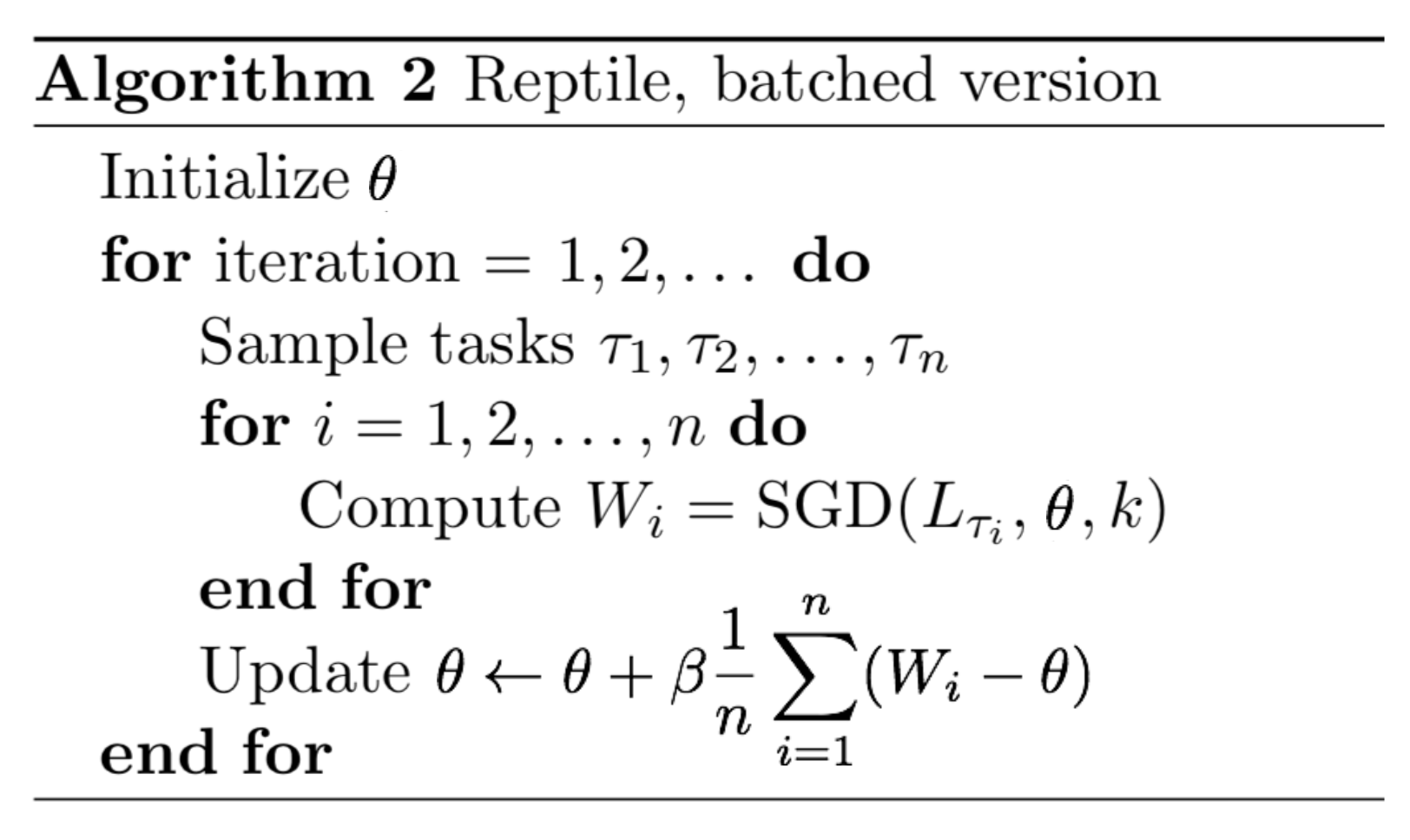
Fig. 13. The batched version of Reptile algorithm. (Image source: original paper)
At a glance, the algorithm looks a lot like an ordinary SGD. However, because the task-specific optimization can take more than one step. it eventually makes \(\text{SGD}(\mathbb{E} _\tau[\mathcal{L}_{\tau}], \theta, k)\) diverge from \(\mathbb{E}_\tau [\text{SGD}(\mathcal{L}_{\tau}, \theta, k)]\) when k > 1.
The Optimization Assumption
Assuming that a task \(\tau \sim p(\tau)\) has a manifold of optimal network configuration, \(\mathcal{W}_{\tau}^*\). The model \(f_\theta\) achieves the best performance for task \(\tau\) when \(\theta\) lays on the surface of \(\mathcal{W}_{\tau}^*\). To find a solution that is good across tasks, we would like to find a parameter close to all the optimal manifolds of all tasks:
\[\theta^* = \arg\min_\theta \mathbb{E}_{\tau \sim p(\tau)} [\frac{1}{2} \text{dist}(\theta, \mathcal{W}_\tau^*)^2]\]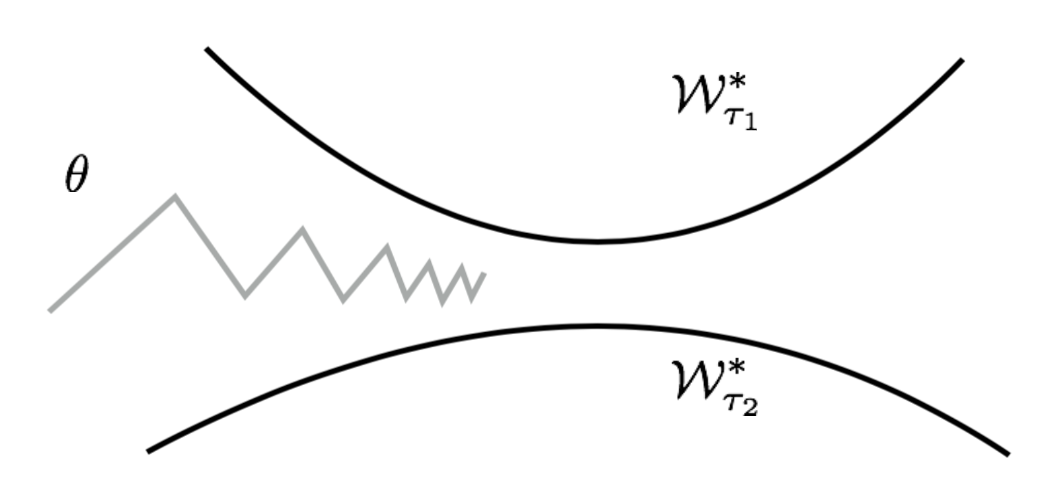
Fig. 14. The Reptile algorithm updates the parameter alternatively to be closer to the optimal manifolds of different tasks. (Image source: original paper)
Let’s use the L2 distance as \(\text{dist}(.)\) and the distance between a point \(\theta\) and a set \(\mathcal{W}_\tau^*\) equals to the distance between \(\theta\) and a point \(W_{\tau}^*(\theta)\) on the manifold that is closest to \(\theta\):
\[\text{dist}(\theta, \mathcal{W}_{\tau}^*) = \text{dist}(\theta, W_{\tau}^*(\theta)) \text{, where }W_{\tau}^*(\theta) = \arg\min_{W\in\mathcal{W}_{\tau}^*} \text{dist}(\theta, W)\]The gradient of the squared euclidean distance is:
\[\begin{aligned} \nabla_\theta[\frac{1}{2}\text{dist}(\theta, \mathcal{W}_{\tau_i}^*)^2] &= \nabla_\theta[\frac{1}{2}\text{dist}(\theta, W_{\tau_i}^*(\theta))^2] & \\ &= \nabla_\theta[\frac{1}{2}(\theta - W_{\tau_i}^*(\theta))^2] & \\ &= \theta - W_{\tau_i}^*(\theta) & \scriptstyle{\text{; See notes.}} \end{aligned}\]Notes: According to the Reptile paper, “the gradient of the squared euclidean distance between a point Θ and a set S is the vector 2(Θ − p), where p is the closest point in S to Θ”. Technically the closest point in S is also a function of Θ, but I’m not sure why the gradient does not need to worry about the derivative of p. (Please feel free to leave me a comment or send me an email about this if you have ideas.)
Thus the update rule for one stochastic gradient step is:
\[\theta = \theta - \alpha \nabla_\theta[\frac{1}{2} \text{dist}(\theta, \mathcal{W}_{\tau_i}^*)^2] = \theta - \alpha(\theta - W_{\tau_i}^*(\theta)) = (1-\alpha)\theta + \alpha W_{\tau_i}^*(\theta)\]The closest point on the optimal task manifold \(W_{\tau_i}^*(\theta)\) cannot be computed exactly, but Reptile approximates it using \(\text{SGD}(\mathcal{L}_\tau, \theta, k)\).
Reptile vs FOMAML
To demonstrate the deeper connection between Reptile and MAML, let’s expand the update formula with an example performing two gradient steps, k=2 in \(\text{SGD}(.)\). Same as defined above, \(\mathcal{L}^{(0)}\) and \(\mathcal{L}^{(1)}\) are losses using different mini-batches of data. For ease of reading, we adopt two simplified annotations: \(g^{(i)}_j = \nabla_{\theta} \mathcal{L}^{(i)}(\theta_j)\) and \(H^{(i)}_j = \nabla^2_{\theta} \mathcal{L}^{(i)}(\theta_j)\).
\[\begin{aligned} \theta_0 &= \theta_\text{meta}\\ \theta_1 &= \theta_0 - \alpha\nabla_\theta\mathcal{L}^{(0)}(\theta_0)= \theta_0 - \alpha g^{(0)}_0 \\ \theta_2 &= \theta_1 - \alpha\nabla_\theta\mathcal{L}^{(1)}(\theta_1) = \theta_0 - \alpha g^{(0)}_0 - \alpha g^{(1)}_1 \end{aligned}\]According to the early section, the gradient of FOMAML is the last inner gradient update result. Therefore, when k=1:
\[\begin{aligned} g_\text{FOMAML} &= \nabla_{\theta_1} \mathcal{L}^{(1)}(\theta_1) = g^{(1)}_1 \\ g_\text{MAML} &= \nabla_{\theta_1} \mathcal{L}^{(1)}(\theta_1) \cdot (I - \alpha\nabla^2_{\theta} \mathcal{L}^{(0)}(\theta_0)) = g^{(1)}_1 - \alpha H^{(0)}_0 g^{(1)}_1 \end{aligned}\]The Reptile gradient is defined as:
\[g_\text{Reptile} = (\theta_0 - \theta_2) / \alpha = g^{(0)}_0 + g^{(1)}_1\]Up to now we have:
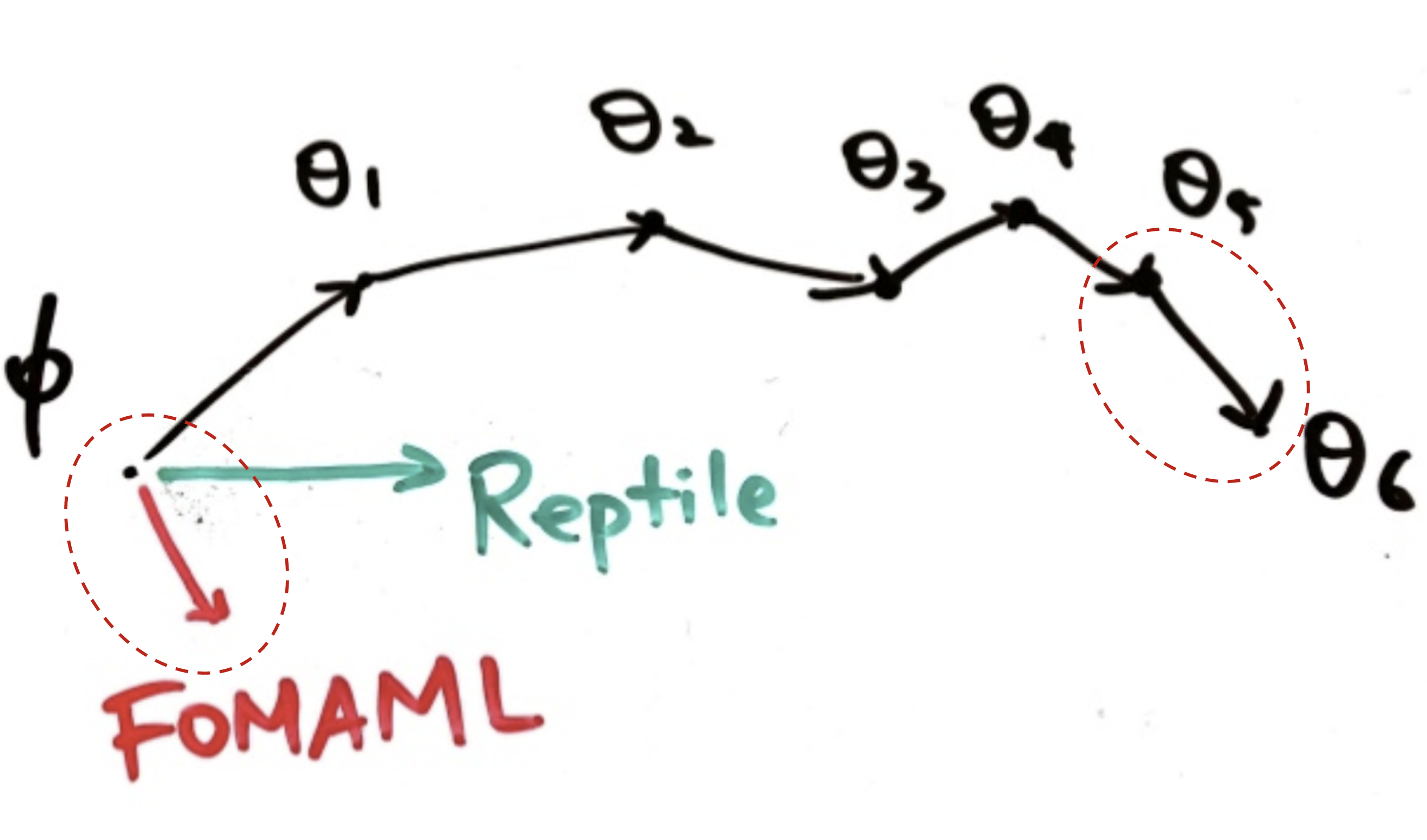
Fig. 15. Reptile versus FOMAML in one loop of meta-optimization. (Image source: slides on Reptile by Yoonho Lee.)
\[\begin{aligned} g_\text{FOMAML} &= g^{(1)}_1 \\ g_\text{MAML} &= g^{(1)}_1 - \alpha H^{(0)}_0 g^{(1)}_1 \\ g_\text{Reptile} &= g^{(0)}_0 + g^{(1)}_1 \end{aligned}\]Next let’s try further expand \(g^{(1)}_1\) using Taylor expansion. Recall that Taylor expansion of a function \(f(x)\) that is differentiable at a number \(a\) is:
\[f(x) = f(a) + \frac{f'(a)}{1!}(x-a) + \frac{f''(a)}{2!}(x-a)^2 + \dots = \sum_{i=0}^\infty \frac{f^{(i)}(a)}{i!}(x-a)^i\]We can consider \(\nabla_{\theta}\mathcal{L}^{(1)}(.)\) as a function and \(\theta_0\) as a value point. The Taylor expansion of \(g_1^{(1)}\) at the value point \(\theta_0\) is:
\[\begin{aligned} g_1^{(1)} &= \nabla_{\theta}\mathcal{L}^{(1)}(\theta_1) \\ &= \nabla_{\theta}\mathcal{L}^{(1)}(\theta_0) + \nabla^2_\theta\mathcal{L}^{(1)}(\theta_0)(\theta_1 - \theta_0) + \frac{1}{2}\nabla^3_\theta\mathcal{L}^{(1)}(\theta_0)(\theta_1 - \theta_0)^2 + \dots & \\ &= g_0^{(1)} - \alpha H^{(1)}_0 g_0^{(0)} + \frac{\alpha^2}{2}\nabla^3_\theta\mathcal{L}^{(1)}(\theta_0) (g_0^{(0)})^2 + \dots & \scriptstyle{\text{; because }\theta_1-\theta_0=-\alpha g_0^{(0)}} \\ &= g_0^{(1)} - \alpha H^{(1)}_0 g_0^{(0)} + O(\alpha^2) \end{aligned}\]Plug in the expanded form of \(g_1^{(1)}\) into the MAML gradients with one step inner gradient update:
\[\begin{aligned} g_\text{FOMAML} &= g^{(1)}_1 = g_0^{(1)} - \alpha H^{(1)}_0 g_0^{(0)} + O(\alpha^2)\\ g_\text{MAML} &= g^{(1)}_1 - \alpha H^{(0)}_0 g^{(1)}_1 \\ &= g_0^{(1)} - \alpha H^{(1)}_0 g_0^{(0)} + O(\alpha^2) - \alpha H^{(0)}_0 (g_0^{(1)} - \alpha H^{(1)}_0 g_0^{(0)} + O(\alpha^2))\\ &= g_0^{(1)} - \alpha H^{(1)}_0 g_0^{(0)} - \alpha H^{(0)}_0 g_0^{(1)} + \alpha^2 \alpha H^{(0)}_0 H^{(1)}_0 g_0^{(0)} + O(\alpha^2)\\ &= g_0^{(1)} - \alpha H^{(1)}_0 g_0^{(0)} - \alpha H^{(0)}_0 g_0^{(1)} + O(\alpha^2) \end{aligned}\]The Reptile gradient becomes:
\[\begin{aligned} g_\text{Reptile} &= g^{(0)}_0 + g^{(1)}_1 \\ &= g^{(0)}_0 + g_0^{(1)} - \alpha H^{(1)}_0 g_0^{(0)} + O(\alpha^2) \end{aligned}\]So far we have the formula of three types of gradients:
\[\begin{aligned} g_\text{FOMAML} &= g_0^{(1)} - \alpha H^{(1)}_0 g_0^{(0)} + O(\alpha^2)\\ g_\text{MAML} &= g_0^{(1)} - \alpha H^{(1)}_0 g_0^{(0)} - \alpha H^{(0)}_0 g_0^{(1)} + O(\alpha^2)\\ g_\text{Reptile} &= g^{(0)}_0 + g_0^{(1)} - \alpha H^{(1)}_0 g_0^{(0)} + O(\alpha^2) \end{aligned}\]During training, we often average over multiple data batches. In our example, the mini batches (0) and (1) are interchangeable since both are drawn at random. The expectation \(\mathbb{E}_{\tau,0,1}\) is averaged over two data batches, ids (0) and (1), for task \(\tau\).
Let,
- \(A = \mathbb{E}_{\tau,0,1} [g_0^{(0)}] = \mathbb{E}_{\tau,0,1} [g_0^{(1)}]\); it is the average gradient of task loss. We expect to improve the model parameter to achieve better task performance by following this direction pointed by \(A\).
- \(B = \mathbb{E}_{\tau,0,1} [H^{(1)}_0 g_0^{(0)}] = \frac{1}{2}\mathbb{E}_{\tau,0,1} [H^{(1)}_0 g_0^{(0)} + H^{(0)}_0 g_0^{(1)}] = \frac{1}{2}\mathbb{E}_{\tau,0,1} [\nabla_\theta(g^{(0)}_0 g_0^{(1)})]\); it is the direction (gradient) that increases the inner product of gradients of two different mini batches for the same task. We expect to improve the model parameter to achieve better generalization over different data by following this direction pointed by \(B\).
To conclude, both MAML and Reptile aim to optimize for the same goal, better task performance (guided by A) and better generalization (guided by B), when the gradient update is approximated by first three leading terms.
\[\begin{aligned} \mathbb{E}_{\tau,1,2}[g_\text{FOMAML}] &= A - \alpha B + O(\alpha^2)\\ \mathbb{E}_{\tau,1,2}[g_\text{MAML}] &= A - 2\alpha B + O(\alpha^2)\\ \mathbb{E}_{\tau,1,2}[g_\text{Reptile}] &= 2A - \alpha B + O(\alpha^2) \end{aligned}\]It is not clear to me whether the ignored term \(O(\alpha^2)\) might play a big impact on the parameter learning. But given that FOMAML is able to obtain a similar performance as the full version of MAML, it might be safe to say higher-level derivatives would not be critical during gradient descent update.
Cited as:
@article{weng2018metalearning,
  title   = "Meta-Learning: Learning to Learn Fast",
  author  = "Weng, Lilian",
  journal = "lilianweng.github.io/lil-log",
  year    = "2018",
  url     = "http://lilianweng.github.io/lil-log/2018/11/29/meta-learning.html"
}
If you notice mistakes and errors in this post, don’t hesitate to leave a comment or contact me at [lilian dot wengweng at gmail dot com] and I would be very happy to correct them asap.
See you in the next post!
Reference
- 【2021-2-7】摘自:awesome-meta-learning
[1] Brenden M. Lake, Ruslan Salakhutdinov, and Joshua B. Tenenbaum. “Human-level concept learning through probabilistic program induction.” Science 350.6266 (2015): 1332-1338.
[2] Oriol Vinyals’ talk on “Model vs Optimization Meta Learning”
[3] Gregory Koch, Richard Zemel, and Ruslan Salakhutdinov. “Siamese neural networks for one-shot image recognition.” ICML Deep Learning Workshop. 2015.
[4] Oriol Vinyals, et al. “Matching networks for one shot learning.” NIPS. 2016.
[5] Flood Sung, et al. “Learning to compare: Relation network for few-shot learning.” CVPR. 2018.
[6] Jake Snell, Kevin Swersky, and Richard Zemel. “Prototypical Networks for Few-shot Learning.” CVPR. 2018.
[7] Adam Santoro, et al. “Meta-learning with memory-augmented neural networks.” ICML. 2016.
[8] Alex Graves, Greg Wayne, and Ivo Danihelka. “Neural turing machines.” arXiv preprint arXiv:1410.5401 (2014).
[9] Tsendsuren Munkhdalai and Hong Yu. “Meta Networks.” ICML. 2017.
[10] Sachin Ravi and Hugo Larochelle. “Optimization as a Model for Few-Shot Learning.” ICLR. 2017.
[11] Chelsea Finn’s BAIR blog on “Learning to Learn”.
[12] Chelsea Finn, Pieter Abbeel, and Sergey Levine. “Model-agnostic meta-learning for fast adaptation of deep networks.” ICML 2017.
[13] Alex Nichol, Joshua Achiam, John Schulman. “On First-Order Meta-Learning Algorithms.” arXiv preprint arXiv:1803.02999 (2018).
[14] Slides on Reptile by Yoonho Lee.
Papers and Code
-
Pytorch版本的MAML实现:How to train your MAML in Pytorch,文章介绍:How to train your MAML: A step by step approach
- Zero-Shot / One-Shot / Few-Shot / Low-Shot Learning
- Siamese Neural Networks for One-shot Image Recognition, (2015), Gregory Koch, Richard Zemel, Ruslan Salakhutdinov. [pdf] [code]
- Prototypical Networks for Few-shot Learning, (2017), Jake Snell, Kevin Swersky, Richard S. Zemel. [pdf] [code]
- Gaussian Prototypical Networks for Few-Shot Learning on Omniglot (2017), Stanislav Fort. [pdf] [code]
- Matching Networks for One Shot Learning, (2017), Oriol Vinyals, Charles Blundell, Timothy Lillicrap, Koray Kavukcuoglu, Daan Wierstra. [pdf] [code]
- Learning to Compare: Relation Network for Few-Shot Learning, (2017), Flood Sung, Yongxin Yang, Li Zhang, Tao Xiang, Philip H.S. Torr, Timothy M. Hospedales. [pdf] [code]
- One-shot Learning with Memory-Augmented Neural Networks, (2016), Adam Santoro, Sergey Bartunov, Matthew Botvinick, Daan Wierstra, Timothy Lillicrap. [pdf] [code]
- Optimization as a Model for Few-Shot Learning, (2016), Sachin Ravi and Hugo Larochelle. [pdf] [code]
- An embarrassingly simple approach to zero-shot learning, (2015), B Romera-Paredes, Philip H. S. Torr. [pdf] [code]
- Low-shot Learning by Shrinking and Hallucinating Features, (2017), Bharath Hariharan, Ross Girshick. [pdf] [code]
- Low-shot learning with large-scale diffusion, (2018), Matthijs Douze, Arthur Szlam, Bharath Hariharan, Hervé Jégou. [pdf] [code]
- Low-Shot Learning with Imprinted Weights, (2018), Hang Qi, Matthew Brown, David G. Lowe. [pdf] [code]
- One-Shot Video Object Segmentation, (2017), S. Caelles and K.K. Maninis and J. Pont-Tuset and L. Leal-Taixe’ and D. Cremers and L. Van Gool. [pdf] [code]
- One-Shot Learning for Semantic Segmentation, (2017), Amirreza Shaban, Shray Bansal, Zhen Liu, Irfan Essa, Byron Boots. [pdf] [code]
- Few-Shot Segmentation Propagation with Guided Networks, (2018), Kate Rakelly, Evan Shelhamer, Trevor Darrell, Alexei A. Efros, Sergey Levine. [pdf] [code]
- Few-Shot Semantic Segmentation with Prototype Learning, (2018), Nanqing Dong and Eric P. Xing. [pdf]
- Dynamic Few-Shot Visual Learning without Forgetting, (2018), Spyros Gidaris, Nikos Komodakis. [pdf] [code]
- Feature Generating Networks for Zero-Shot Learning, (2017), Yongqin Xian, Tobias Lorenz, Bernt Schiele, Zeynep Akata. [pdf]
- Meta-Learning Deep Visual Words for Fast Video Object Segmentation, (2019), Harkirat Singh Behl, Mohammad Najafi, Anurag Arnab, Philip H.S. Torr. [pdf]
- Model Agnostic Meta Learning
- Model-Agnostic Meta-Learning for Fast Adaptation of Deep Networks, (2017), Chelsea Finn, Pieter Abbeel, Sergey Levine. [pdf] [code]
- Adversarial Meta-Learning, (2018), Chengxiang Yin, Jian Tang, Zhiyuan Xu, Yanzhi Wang. [pdf] [code]
- On First-Order Meta-Learning Algorithms, (2018), Alex Nichol, Joshua Achiam, John Schulman. [pdf] [code]
- Meta-SGD: Learning to Learn Quickly for Few-Shot Learning, (2017), Zhenguo Li, Fengwei Zhou, Fei Chen, Hang Li. [pdf] [code]
- Gradient Agreement as an Optimization Objective for Meta-Learning, (2018), Amir Erfan Eshratifar, David Eigen, Massoud Pedram. [pdf] [code]
- Gradient-Based Meta-Learning with Learned Layerwise Metric and Subspace, (2018), Yoonho Lee, Seungjin Choi. [pdf] [code]
- A Simple Neural Attentive Meta-Learner, (2018), Nikhil Mishra, Mostafa Rohaninejad, Xi Chen, Pieter Abbeel. [pdf] [code]
- Personalizing Dialogue Agents via Meta-Learning, (2019), Zhaojiang Lin, Andrea Madotto, Chien-Sheng Wu, Pascale Fung. [pdf] [code]
- How to train your MAML, (2019), Antreas Antoniou, Harrison Edwards, Amos Storkey. [pdf] [code]
- Learning to learn by gradient descent by gradient descent, (206), Marcin Andrychowicz, Misha Denil, Sergio Gomez, Matthew W. Hoffman, David Pfau, Tom Schaul, Brendan Shillingford, Nando de Freitas. [pdf] [code]
- Unsupervised Learning via Meta-Learning, (2019), Kyle Hsu, Sergey Levine, Chelsea Finn. [pdf] [code]
- Few-Shot Image Recognition by Predicting Parameters from Activations, (2018), Siyuan Qiao, Chenxi Liu, Wei Shen, Alan Yuille. [pdf] [code]
- One-Shot Imitation from Observing Humans via Domain-Adaptive Meta-Learning, (2018), Tianhe Yu, Chelsea Finn, Annie Xie, Sudeep Dasari, Pieter Abbeel, Sergey Levine, [pdf] [code]
- MetaGAN: An Adversarial Approach to Few-Shot Learning, (2018), ZHANG, Ruixiang and Che, Tong and Ghahramani, Zoubin and Bengio, Yoshua and Song, Yangqiu. [pdf]
- Fast Parameter Adaptation for Few-shot Image Captioning and Visual Question Answering,(2018), Xuanyi Dong, Linchao Zhu, De Zhang, Yi Yang, Fei Wu. [pdf]
- CAML: Fast Context Adaptation via Meta-Learning, (2019), Luisa M Zintgraf, Kyriacos Shiarlis, Vitaly Kurin, Katja Hofmann, Shimon Whiteson. [pdf]
- Meta-Learning for Low-resource Natural Language Generation in Task-oriented Dialogue Systems, (2019), Fei Mi, Minlie Huang, Jiyong Zhang, Boi Faltings. [pdf]
- MIND: Model Independent Neural Decoder, (2019), Yihan Jiang, Hyeji Kim, Himanshu Asnani, Sreeram Kannan. [pdf]
- Toward Multimodal Model-Agnostic Meta-Learning, (2018), Risto Vuorio, Shao-Hua Sun, Hexiang Hu, Joseph J. Lim. [pdf]
- Alpha MAML: Adaptive Model-Agnostic Meta-Learning, (2019), Harkirat Singh Behl, Atılım Güneş Baydin, Philip H. S. Torr. [pdf]
- Online Meta-Learning, (2019), Chelsea Finn, Aravind Rajeswaran, Sham Kakade, Sergey Levine. [pdf]
- Meta Reinforcement Learning
- Generalizing Skills with Semi-Supervised Reinforcement Learning, (2017), Chelsea Finn, Tianhe Yu, Justin Fu, Pieter Abbeel, Sergey Levine. [pdf] [code]
- Guided Meta-Policy Search, (2019), Russell Mendonca, Abhishek Gupta, Rosen Kralev, Pieter Abbeel, Sergey Levine, Chelsea Finn. [pdf] [code]
- End-to-End Robotic Reinforcement Learning without Reward Engineering, (2019), Avi Singh, Larry Yang, Kristian Hartikainen, Chelsea Finn, Sergey Levine. [pdf] [code]
- Efficient Off-Policy Meta-Reinforcement Learning via Probabilistic Context Variables, (2019), Kate Rakelly, Aurick Zhou, Deirdre Quillen, Chelsea Finn, Sergey Levine. [pdf] [code]
- Meta-Gradient Reinforcement Learning, (2018), Zhongwen Xu, Hado van Hasselt,David Silver. [pdf]
- Task-Agnostic Dynamics Priors for Deep Reinforcement Learning, (2019), Yilun Du, Karthik Narasimhan. [pdf]
- Meta Reinforcement Learning with Task Embedding and Shared Policy,(2019), Lin Lan, Zhenguo Li, Xiaohong Guan, Pinghui Wang. [pdf]
- NoRML: No-Reward Meta Learning, (2019), Yuxiang Yang, Ken Caluwaerts, Atil Iscen, Jie Tan, Chelsea Finn. [pdf]
- Actor-Critic Algorithms for Constrained Multi-agent Reinforcement Learning, (2019), Raghuram Bharadwaj Diddigi, Sai Koti Reddy Danda, Prabuchandran K. J., Shalabh Bhatnagar. [pdf]
- Adaptive Guidance and Integrated Navigation with Reinforcement Meta-Learning, (2019), Brian Gaudet, Richard Linares, Roberto Furfaro. [pdf]
- Watch, Try, Learn: Meta-Learning from Demonstrations and Reward, (2019), Allan Zhou, Eric Jang, Daniel Kappler, Alex Herzog, Mohi Khansari, Paul Wohlhart, Yunfei Bai, Mrinal Kalakrishnan, Sergey Levine, Chelsea Finn. [pdf]
- Options as responses: Grounding behavioural hierarchies in multi-agent RL, (2019), Alexander Sasha Vezhnevets, Yuhuai Wu, Remi Leblond, Joel Z. Leibo. [pdf]
- Learning latent state representation for speeding up exploration, (2019), Giulia Vezzani, Abhishek Gupta, Lorenzo Natale, Pieter Abbeel. [pdf]
- Beyond Exponentially Discounted Sum: Automatic Learning of Return Function, (2019), Yufei Wang, Qiwei Ye, Tie-Yan Liu. [pdf]
- Learning Efficient and Effective Exploration Policies with Counterfactual Meta Policy, (2019), Ruihan Yang, Qiwei Ye, Tie-Yan Liu. [pdf]
- Dealing with Non-Stationarity in Multi-Agent Deep Reinforcement Learning, (2019), Georgios Papoudakis, Filippos Christianos, Arrasy Rahman, Stefano V. Albrecht. [pdf]
-
Learning to Discretize: Solving 1D Scalar Conservation Laws via Deep Reinforcement Learning, (2019), Yufei Wang, Ziju Shen, Zichao Long, Bin Dong. [pdf]
- Meta-Dataset: A Dataset of Datasets for Learning to Learn from Few Examples. Eleni Triantafillou, Tyler Zhu, Vincent Dumoulin, Pascal Lamblin, Kelvin Xu, Ross Goroshin, Carles Gelada, Kevin Swersky, Pierre-Antoine Manzagol, Hugo Larochelle.
- Gradient-Based Meta-Learning with Learned Layerwise Metric and Subspace. Yoonho Lee, Seungjin Choi.

- FIGR: Few-shot Image Generation with Reptile. Louis Clouâtre, Marc Demers.
- Online gradient-based mixtures for transfer modulation in meta-learning. Ghassen Jerfel, Erin Grant, Thomas L. Griffiths, Katherine Heller.
- Auto-Meta: Automated Gradient Based Meta Learner Search. Jaehong Kim, Youngduck Choi, Moonsu Cha, Jung Kwon Lee, Sangyeul Lee, Sungwan Kim, Yongseok Choi, Jiwon Kim.
- MetaGAN: An Adversarial Approach to Few-Shot Learning. ZHANG, Ruixiang and Che, Tong and Ghahramani, Zoubin and Bengio, Yoshua and Song, Yangqiu.
- Learned Optimizers that Scale and Generalize. Olga Wichrowska, Niru Maheswaranathan, Matthew W. Hoffman, Sergio Gomez Colmenarejo, Misha Denil, Nando de Freitas, Jascha Sohl-Dickstein.
- Guiding Policies with Language via Meta-Learning. John D. Co-Reyes, Abhishek Gupta, Suvansh Sanjeev, Nick Altieri, John DeNero, Pieter Abbeel, Sergey Levine.
- Deep Comparison: Relation Columns for Few-Shot Learning. Xueting Zhang, Flood Sung, Yuting Qiang, Yongxin Yang, Timothy M. Hospedales.
- Towards learning-to-learn. Benjamin James Lansdell, Konrad Paul Kording.
- Learning to Learn with Gradients. Finn, Chelsea.
- How to train your MAML. Antreas Antoniou, Harrison Edwards, Amos Storkey.
- Learned optimizers that outperform SGD on wall-clock and validation loss. Luke Metz, Niru Maheswaranathan, Jeremy Nixon, C. Daniel Freeman, Jascha Sohl-Dickstein
- Gradient Agreement as an Optimization Objective for Meta-Learning. Amir Erfan Eshratifar, David Eigen, Massoud Pedram.
- Few-Shot Image Recognition by Predicting Parameters from Activations. Siyuan Qiao, Chenxi Liu, Wei Shen, Alan Yuille. CVPR 2018.
- META-LEARNING WITH LATENT EMBEDDING OPTIMIZATION. Andrei A. Rusu, Dushyant Rao, Jakub Sygnowski, Oriol Vinyals, Razvan Pascanu, Simon Osindero & Raia Hadsell
- Model-Agnostic Meta-Learning for Fast Adaptation of Deep Networks, Chelsea Finn, Pieter Abbeel, Sergey Levine. ICML 2017.
- On First-Order Meta-Learning Algorithms. Alex Nichol, Joshua Achiam, John Schulman.
- Prototypical Networks for Few-shot Learning, Jake Snell, Kevin Swersky, Richard S. Zemel. NIPS 2017.
- Learning to learn by gradient descent by gradient descent, Marcin Andrychowicz, Misha Denil, Sergio Gomez, Matthew W. Hoffman, David Pfau, Tom Schaul, Brendan Shillingford, Nando de Freitas
- Learning to Learn without Gradient Descent by Gradient Descent, Yutian Chen, Matthew W. Hoffman, Sergio Gomez Colmenarejo, Misha Denil, Timothy P. Lillicrap, Matt Botvinick, Nando de Freitas, ICML 2017
- OPTIMIZATION AS A MODEL FOR FEW-SHOT LEARNING, Sachin Ravi, Hugo Larochelle. ICLR 2017
- Meta-SGD: Learning to Learn Quickly for Few-Shot Learning, Zhenguo Li, Fengwei Zhou, Fei Chen, Hang Li
- Unsupervised Meta-Learning for Reinforcement Learning. Abhishek Gupta, Benjamin Eysenbach, Chelsea Finn, Sergey Levine.
- Learning to Compare: Relation Network for Few-Shot Learning, Flood Sung, Yongxin Yang, Li Zhang, Tao Xiang, Philip H.S. Torr, Timothy M. Hospedales, CVPR 2018
Few-shot Pytorch
Zero-shot Pytorch
miniImageNet Pytorch
- Object-Level Representation Learning for Few-Shot Image Classification, Liangqu Long, Wei Wang, Jun Wen, Meihui Zhang, Qian Lin, Beng Chin Ooi
- A Simple Neural Attentive Meta-Learner, Nikhil Mishra, Mostafa Rohaninejad, Xi Chen, Pieter Abbeel. ICLR 2018
- Meta-Learning for Semi-Supervised Few-Shot Classification, Mengye Ren, Eleni Triantafillou, Sachin Ravi, Jake Snell, Kevin Swersky, Joshua B. Tenenbaum, Hugo Larochelle, Richard S. Zemel. ICLR 2018,提出一种新的extensions of Prototypical Networks
- Learning to Optimize, Ke Li, Jitendra Malik
- Matching Networks for One Shot Learning, Oriol Vinyals, Charles Blundell, Timothy Lillicrap, Koray Kavukcuoglu, Daan Wierstra
- Meta-Learning with Memory-Augmented Neural Networks, Adam Santoro, Sergey Bartunov, Matthew Botvinick, Daan Wierstra, Timothy Lillicrap
- CAML: Fast Context Adaptation via Meta-Learning, Luisa M Zintgraf, Kyriacos Shiarlis, Vitaly Kurin, Katja Hofmann, Shimon Whiteson
- Unsupervised Learning via Meta-Learning, Kyle Hsu, Sergey Levine, Chelsea Finn
- Fast Parameter Adaptation for Few-shot Image Captioning and Visual Question Answering. Xuanyi Dong, Linchao Zhu, De Zhang, Yi Yang, Fei Wu.
Tutorials and Slides
- NeuraIPS meta-learning workshop: 2018, 2017
- What’s Wrong with Meta-Learning
- Meta-Learning: Learning to Learn Fast
- How to train your MAML: A step by step approach
- From zero to research — An introduction to Meta-learning
- Deep learning to learn. Pieter Abbeel
- Meta-Learning Frontiers: Universal, Uncertain, and Unsupervised, Sergey Levine, Chelsea Finn
Blogs
- Berkeley Artificial Intelligence Research blog
- Meta-Learning: Learning to Learn Fast
- Meta-Reinforcement Learning
- How to train your MAML: A step by step approach
- An Introduction to Meta-Learning
- From zero to research — An introduction to Meta-learning
- What’s New in Deep Learning Research: Understanding Meta-Learning
- Meta Reinforcement Learning Blog by Lilian Weng
Lecture Videos
- Stanford CS330: Multi-Task and Meta-Learning, 2019 by Chelsea Finn
- Meta Learning lecture by Soheil Feizi
- Chelsea Finn: Building Unsupervised Versatile Agents with Meta-Learning
- Sam Ritter: Meta-Learning to Make Smart Inferences from Small Data
- Model Agnostic Meta Learning by Siavash Khodadadeh
- Meta Learning by Siraj Raval
- Meta Learning by Hugo Larochelle
- Meta Learning and One-Shot Learning
Workshops
Reseachers and Labs
Libraries
Labs
- Chelsa Finn, UC Berkeley
- Misha Denil, DeepMind
- Sachin Ravi, Princeton University
- Hugo Larochelle, Google Brain
- Jake Snell, University of Toronto, Vector Institute
- Adam Santoro, DeepMind
- JANE X. WANG, DeepMind
Researchers
- Chelsea Finn, UC Berkeley
- Pieter Abbeel, UC Berkeley
- Erin Grant, UC Berkeley
- Raia Hadsell, DeepMind
- Misha Denil, DeepMind
- Adam Santoro, DeepMind
- Sachin Ravi, Princeton University
- David Abel, Brown University
- Brenden Lake, Facebook AI Research
 支付宝打赏
支付宝打赏  微信打赏
微信打赏